In portfolio management, Value-at-Risk (VaR) is a popular metric to quantitatively assess the risk of our holdings.
Originally invented by banks to give some sense to how much lost could be reasonably anticipated across different business, it gained traction in the risk management world and soon become a well-known method to measuring risk and helping traders/portfolio managers to view their portfolio in a different fashion.
Today let’s learn about what is VaR, and how we can compute it in Excel.
You may also be interested in 2021 New Year Resolution List for Excel.
Workbook
What is Value-at-Risk (VaR)?
Value-at-Risk (VaR) is, in essence, the X-percentile of the projected Profit-and-loss (PnL) for our portfolio, over a given time horizon. In plain words, if VaR is $100, it tells you that if we are unlucky tomorrow, we expect to lose at a maximum of $100 with X% chance/confidence.
Let’s think about it in a non-financial example. Suppose you have 99 students in a Mathematics class, taking the same test tomorrow. Based on the result of the last test they’ve taken, you obtained a projection of how the class will perform in the coming test.
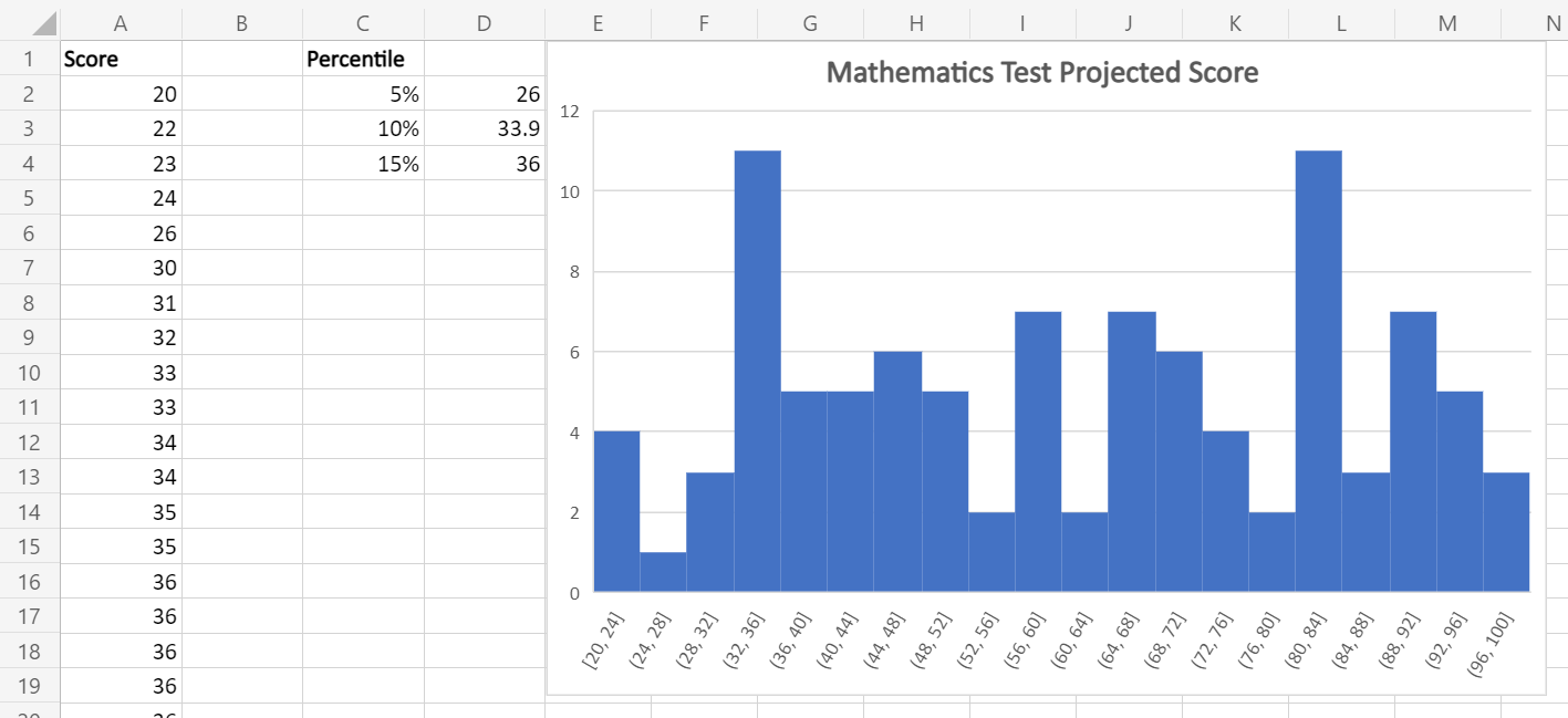
With the data in our example workbook, we found that the 5th percentile of the score is at 26, which is basically the 5th-lowest score achieved by the class (cell A6). Therefore, we can loosely say that the 5% Value-at-Risk for the class is 26 in the upcoming test, i.e. we have 5% confidence that the lowest score achieved by all students is 26.
You may also be interested in Binomial Option Pricing (Excel formula).
Why do we use Value-at-Risk (VaR)?
Now let’s turn our attention to portfolios of financial instruments. Instead of the score of students, now we look to project the Profit-and-Loss (PnL) of our portfolio, and compute a Value-at-Risk (VaR) based on that.
There are actually good reason to look at Value-at-Risk (VaR), on top of usual metrics like expected return/portfolio standard deviation. VaR is actually a metric to look at heavy-tail events (or black-swan events).

Heavy-tail (or black-swan) events are rare events that have severe consequence. For example, people generally think the stock market would not drop by more than 5% a day, so “Market dropping by more than 5%” is a black-swan event.
While metrics like expected return/portfolio standard deviation give investor a sense of the characteristics of their portfolio, they do not tell you what could happen if you have a really bad day. And VaR is a good metric to tell you that, if you have a really bad day, what is the loss to be expected.
For large investor, heavy-tail events are risks to be managed, and hence heavy-tail metrics like VaR has grown in prominence for risk management.
With this in mind, our problem becomes:
- How do we present VaR figures?
- How do we come up with the statistical distribution of the PnL (i.e. the chances of achieving different PnL levels)?
Let’s go through one-by-one in the following section.
You may also be interested in How to Compute IRR in Excel (Basic to Advanced).
How do we present Value-at-Risk (VaR)?
In practice, Value-at-Risk (VaR) often comes in different flavors, and it is important for us to understand how to read into the VaR figures provided.
Confidence Level
VaR is always presented in the manner “X%-VaR“, and we specify the confidence level (i.e. X%) related to a specific VaR. For example, a 95%-VaR would correspond to the 5th-percentile of the PnL distribution, 99%-VaR to the 1st-percentile of the PnL distribution.
There is no one-shoe-fit-all rule that dictates what is the confidence level to use, but practitioners generally quotes multiple confidence level at once (e.g. 95%, 97.5%, 99%) to give a better sense for how heavy-tail events would impact the portfolio.
Time Horizon
VaR is also commonly presented as a “X-day VaR“, although sometimes it is implicitly a 1-day VaR measure. When speaking of the PnL distribution, depending on the frequency of the data (e.g. daily/weekly/monthly), VaR of different time horizon could be calculated.
Majority of the VaR measures in practice is a 1-day metric, as a typical assumption is that risks are reviewed on a daily basis, but longer horizon metrics are often useful as well.
Absolute vs Relative
Absolute and Relative VaR differs in whether you want to benchmark against the expected return.
For example, suppose the 5th percentile of your PnL distribution is -$10, and your expected return (i.e. mean of PnL distribution) is +$2. Your Absolute 95%-VaR would be -$10 (the total loss expected), and your Relative 95%-VaR would be -$8 (a relative figure to the expected return).
You may also be interested in How to Generate Random Variables in Excel.
How do we come up with the statistical distribution?
After we discussed on what are the flavors for Value-at-Risk (VaR), we look at a more fundamental question – how do we come up with the distribution of potential Profit-and-Loss (PnL) in the first place?
Ultimately, the computed VaR depends on your selected PnL distribution: if you select a distribution that there is a high chance of losing (positively skewed), chances are, your VaR computed will be larger than if you have picked a distribution that is more symmetrical.
There are mainly 2 ways which we’ll illustrate with the help of Excel:
- Historical approach
- Parametric approach
Historical Approach
As the name suggest, in historical approach, you compute the VaR based on what is available in the past.
In essence, based on the specific portfolio composition, we obtain the daily PnL data, sort them in ascending order, and find the relevant (1-X)-th percentile that translates to our X%-VaR.
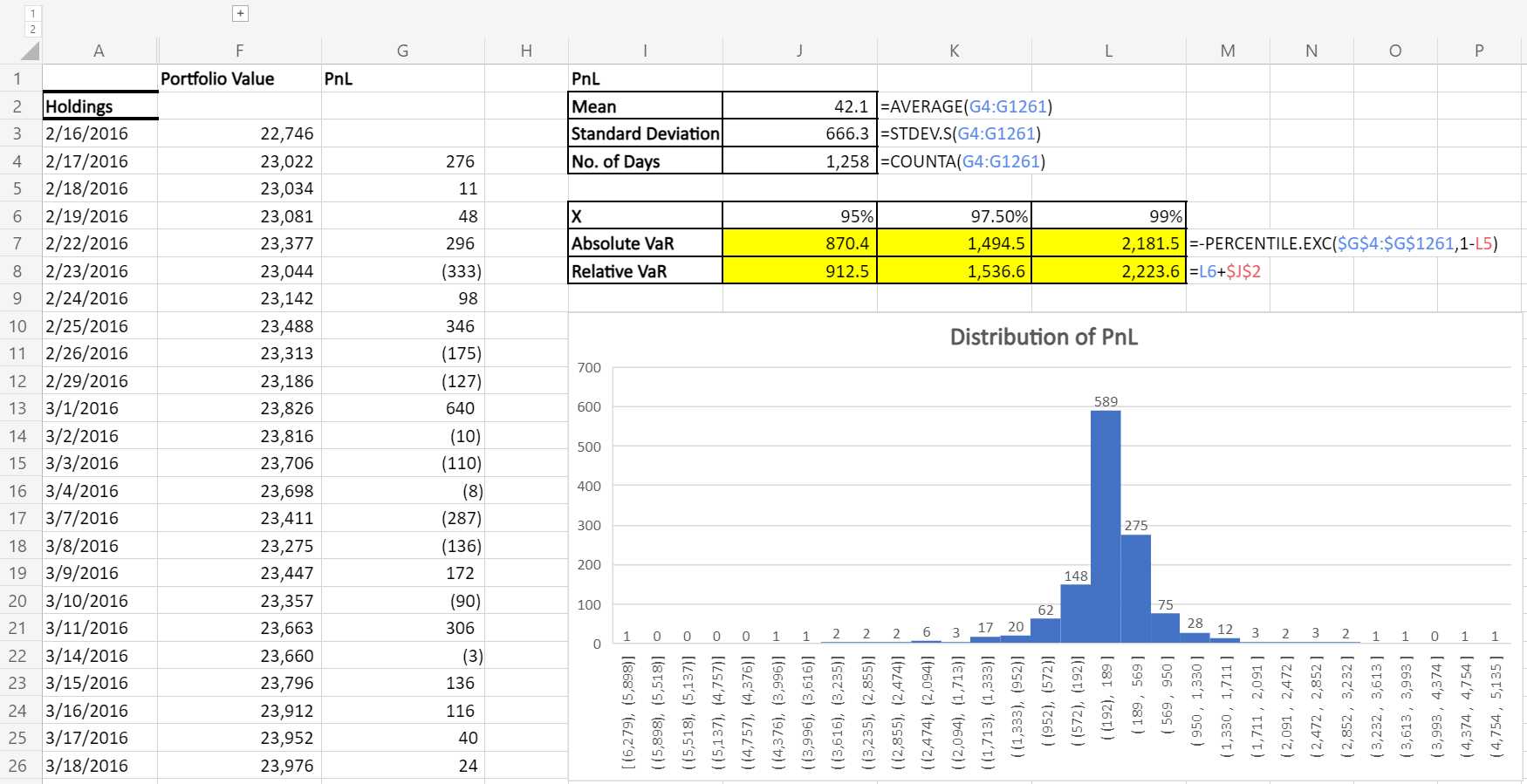
From the Sample Workbook, you’ll find an example where we have a portfolio with 4 stocks. With Yahoo Finance stock price data, we compute the day-on-day change as our PnL distribution.
Based on the calculation, we found that the 1-day 95%-VaR is $870.4, which means on a given day, we expect that the maximum loss is $870.4 with 5% confidence. Similarly we have the 97.5%-VaR and 99%-VaR for side-by-side comparison.
As you’ve guessed, there are several limitation of using a historical approach:
- The computed VaR is heavily influenced by the timeframe you’ve selected.
- Past performance of the portfolio does not necessarily link closely to future performance
- Most importantly, sampling of the negative outliers (i.e. days with large loss) may be biased as we usually have too few observations.
With that in mind, we introduce the alternative approach: the parametric approach.
You may also be interested in Black-Scholes Option Pricing (Excel formula).
Parametric Approach
The parametric approach is a fancy way to say that we make some statistical assumption with the PnL distribution.
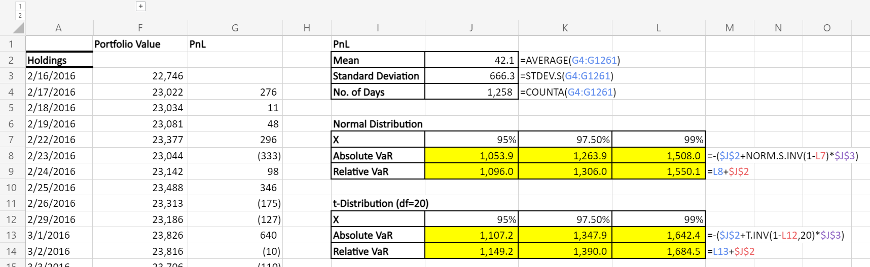
For example, in our sample workbook, we’ve presented VaR computed from 2 commonly-used parametric distribution: the Normal distribution and the t-distribution.
In the Parametric Approach, we only need to estimate for a couple of parameters (e.g. mean and standard deviation) of the PnL distribution, and apply these parameter to find the expected percentile.
Notice how the VaR computed for t-distribution is larger than the normal distribution, which is due to the fact that t-distribution has heavier tails than the normal distribution. Heavier tail means that there are more chances for outliers (negative outcome in our case).
Comparing what we computed in parametric vs historical approach, while parametric approach seems more prudent than the historical approach for 95%-VaR (1,053.9 vs 870.4, larger means more prudent), for 99%-VaR (1,508.0 vs 2,181.5) the opposite is true.
In this case, we’ll need to re-evaluate whether our choice of parametric PnL distribution (e.g. Normal/t) is representative of the actual PnL distribution, and see if we need to find a more heavy-tailed distribution.
You may also be interested in How to Name Multiple Single Cells in Excel.
Bottomline
Value-at-Risk (VaR) is an important metric in risk management, giving investors/traders the sense of how heavy-tail/black-swan events would impact the portfolio of financial instruments we hold.
There are numerous ways to how VaR can be computed and presented, but we should always compare and contrast VaR computed with different approach and understand what it means for our modelling and how it could be representative of our risks.
You may be interested in How to use REPT functions to the Most.
Hungry for more useful Excel tips like this? Subscribe to our newsletter to make sure you won’t miss out on any of our posts and get exclusive Excel tips!