


I have a drop-down list and I want the cell to be formatted to a specific color depending on the selected value.
Numerous Excel users
From time to time, I get this questions from my followers on Instagram.
They want the cell to change colour when certain value is selected from the drop-down list.
This sounds a bit complicated but it’s actually quite simple.
In this article, I will show you how to auto change colour of the cell based on the selected value from drop down list.
Example
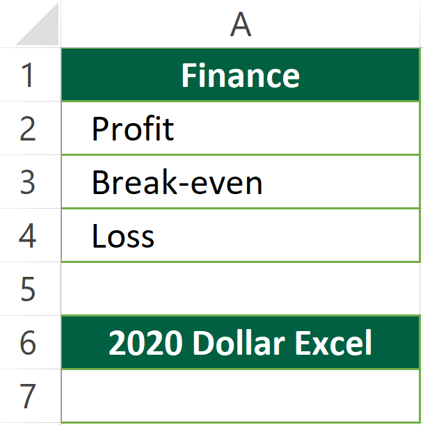
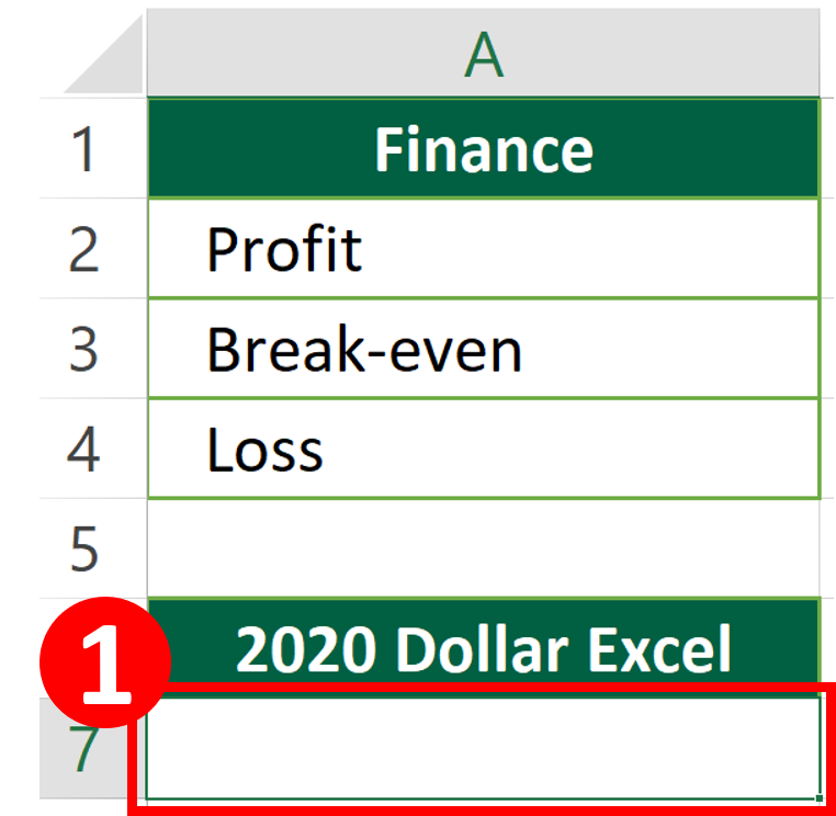
There are 3 financial situations, which are Profit, break-even and loss respectively.
Sample Workbook
Download the workbook to practice it by yourself!

Expected Outcome
In this article, I will show you how to make a drop down list with colours.
Indeed, we will be using data validation and conditional formatting.
Step 1: Select cells to validate
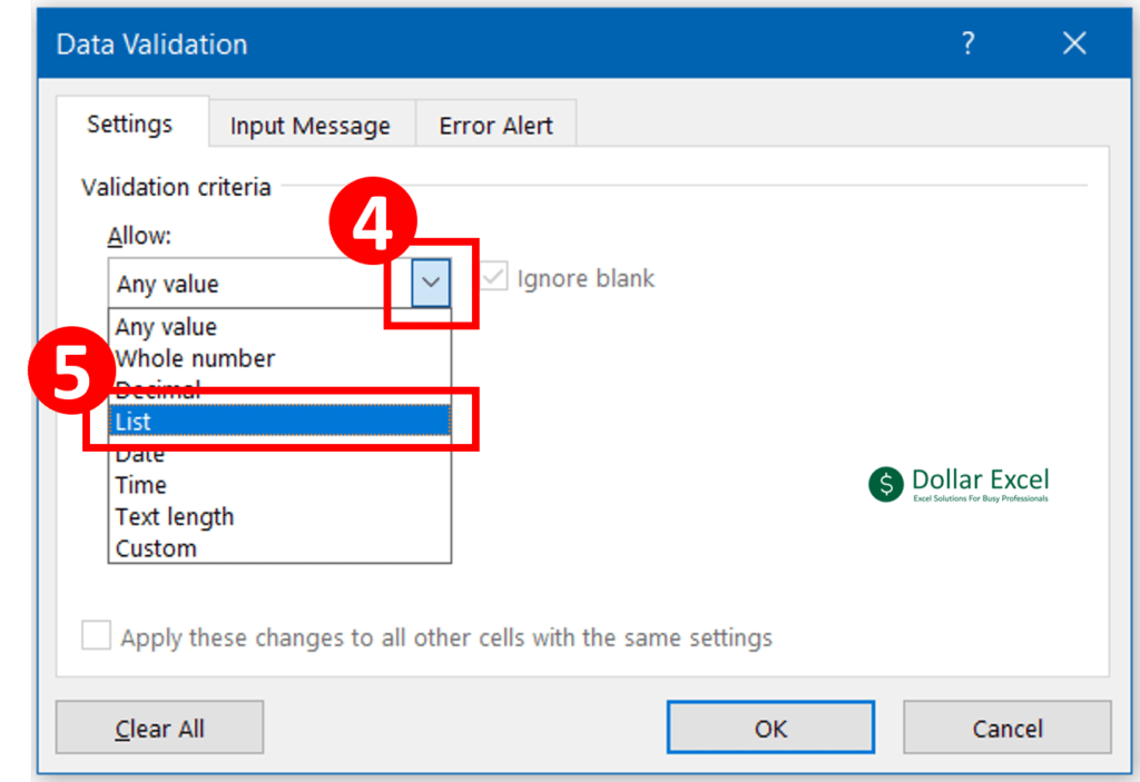
Step 2-3: In Data tab, select data validation

Step 4-5: Press the small triangle, select List
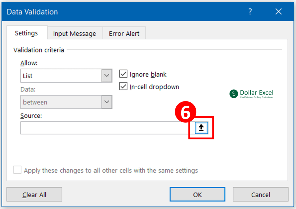
Step 6: Press the small triangle, select List
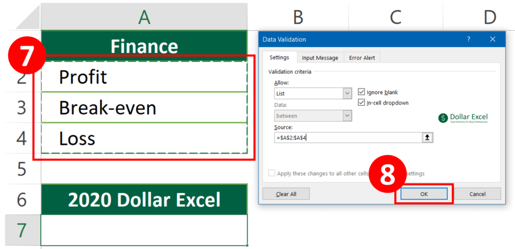
Step 7-8: Select the source for data validation and press OK
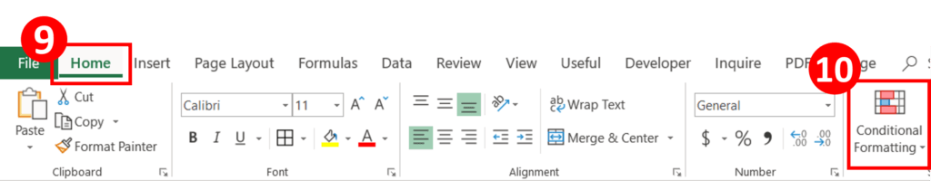
Step 9-10: In home tab, select Conditional Formatting
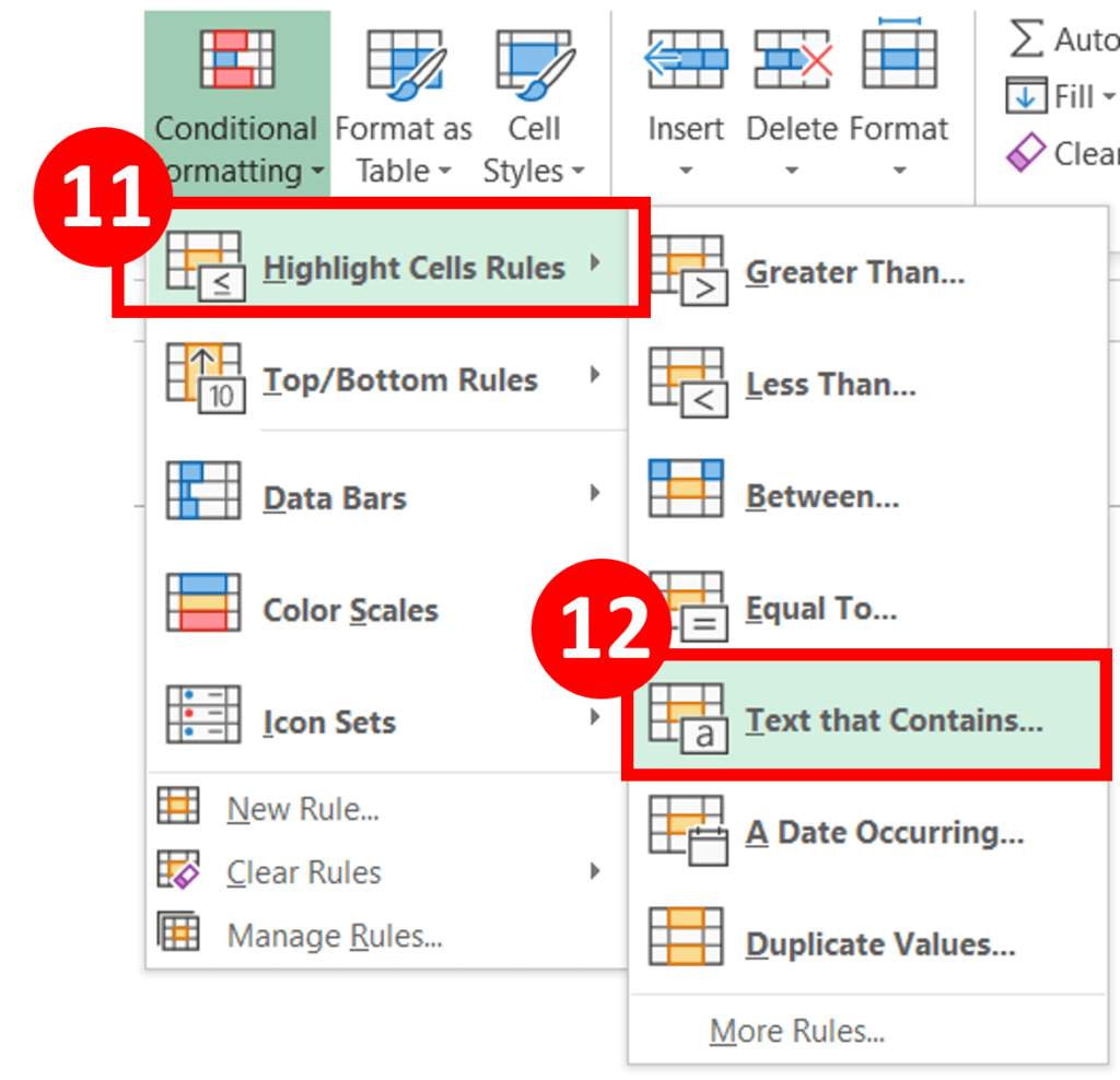
Step 11-12: Select “Highlight Cells Rules” and “Text that Contains…”
Step 13-14: Select “Highlight Cells Rules” and “Text that Contains…”
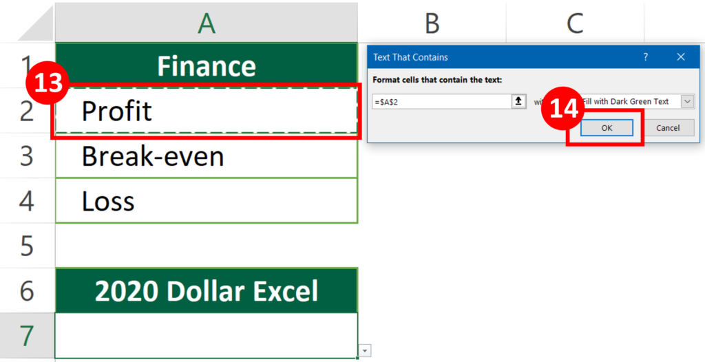
Step 15: Repeat step 13-14 for the “Breakeven” and “Loss”
Step 16: Done
Do you find this article helpful? Subscribe to our newsletter to get exclusive Excel tips!