
Background
Named range is a very useful feature in Excel.
With Named range, the formula is more dynamic and looks a lot more descriptive.
However, naming range itself can be a painful process.
Naming 50 ranges manually can take you half an hour’s time.
Do you know you can actually name a bunch of ranges in a few clicks with a cool Excel feature?
- How to name multiple single cells in Excel?
- How to name multiple ranges in Excel?
- How to name ranges efficiently in Excel?
- How to name cells in bulk in Excel?
In this article, I will show you how to name multiple cells in Excel step-by-step using a cool feature called “Create from Selection”. With this, you can easily create a hundred of named range in a few seconds.
Sample Workbook
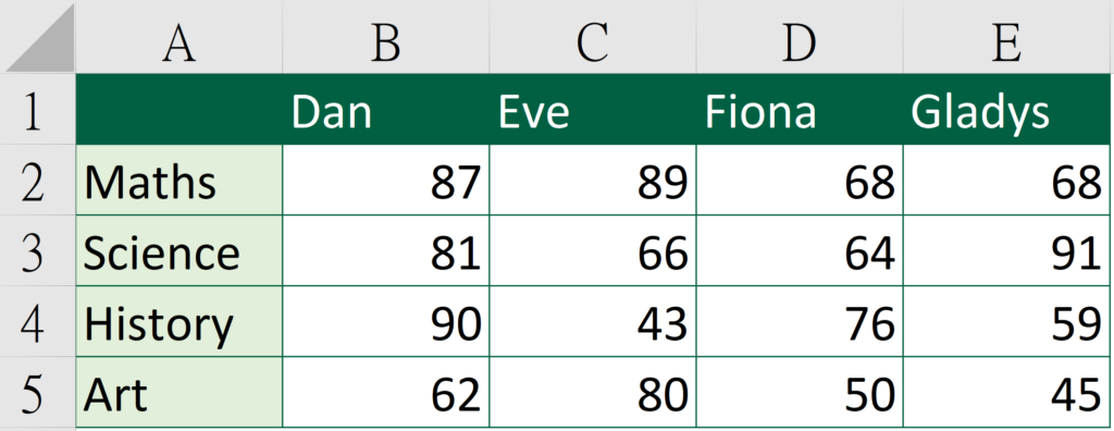
In this article, I will use the following table as an example.
Download the workbook to practice it by yourself!
Press the download button!

Step-by-step Tutorial
Before we start the tutorial, there are some prerequisites that you need to keep in mind.
To be able to follow the tutorial, you need to make sure it follows the below format.
It should look like a table, rather than some messy cell ranges.
The column header should locate either on the top of the table or at the bottom.
The row header should locate either on the leftmost column or the rightmost column.
You don’t need both column header and row header but you need at least one.
In this tutorial, I will demonstrate with both column and row header for illustration purpose.
Step 1: Select the range you would like to name

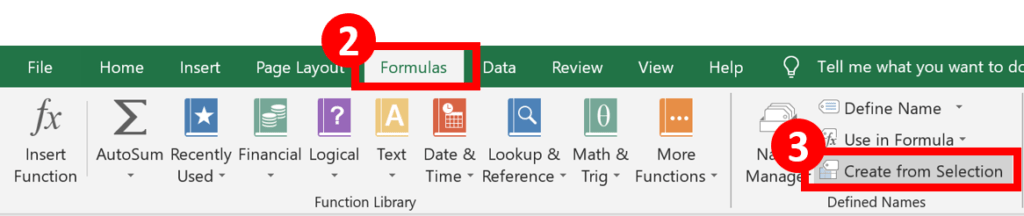
Step 2-3: On the “Formulas” tab, select “Create from Selection”
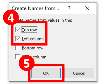
Step 4-5: In the “Create Names from Selection” dialog, check the appropriate box and press “OK”
In this example, I put the column header at the first row of the selection so I am gonna check the “Top row” box. Since I put the row title on the leftmost column, I am also gonna select “Left column”.
Actually, very likely Excel has already check the box for you. Just make sure it is checking the box you want or things might go wrong.
Check the named ranges
Now you have already named multiple ranges.
Don’t believe it? Let’s open the “Name Manager” dialog and check whether those names are there.
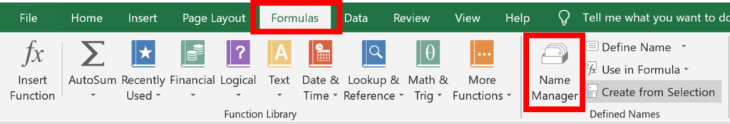
On the Formulas tab, select Name Manager.
Then the “Name Manager” dialog will pop up.
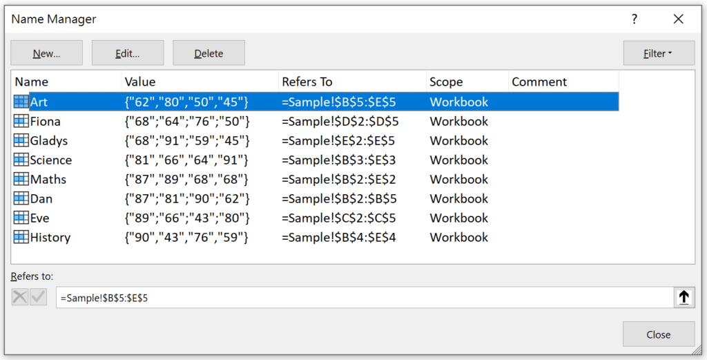
As you can see from the dialog, now we have got 8 named ranges, each named with either the column header or the row header.
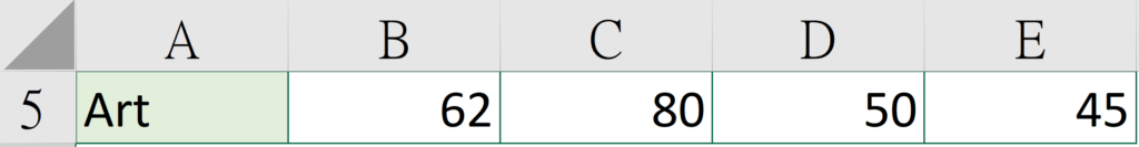
For example, the named range “Art” contains {“62”, “80”, “50”, “45”}, which are the values of Cell B5, Cell C5, Cell D5 and Cell E5 respectively.
Demonstration of the usage of Named ranges
To make the formula more descriptive
We learned how to name multiple ranges efficiently.
Yet, why would we need to name a range in the first place?
Below I will demonstrate the usage of named ranges.
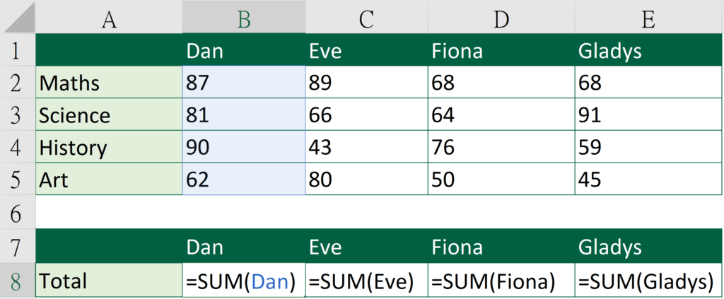
In the below example, row 8 sums the total score of each students.
Very often when we want to sum ranges, we would simply put =sum(ranges).
For example, the usual formula to sum Dan’s score will be like this.
=SUM(B2:B5)
There is nothing wrong with this formula.
However, when we are looking for a more descriptive formula, we can do this one instead.
=SUM(Dan)
By looking at the formula alone, you know what the formula is for and what kind of references it took into.
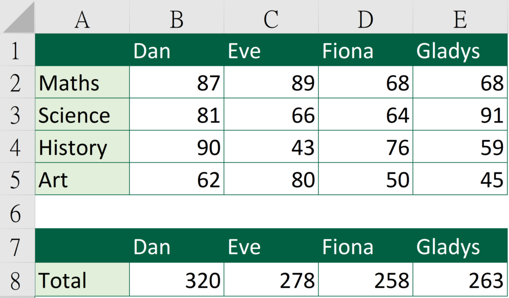
Here is the result.
To work like a look up tool
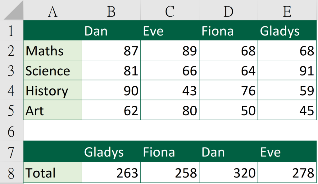
In order to show the difference, I change the order of the names a bit.
Originally, the order is Dan > Eve > Fiona > Gladys
Now, the order becomes Gladys > Fiona > Dan > Eve
So it is kind of like a mini look up tool rather than a simple sum.
How to achieve that?
Formula of Cell B8:
=SUM(INDIRECT(B7))
In the formula, I used INDIRECT function. Read This article to know more about INDIRECT function.
The INDIRECT function allows me to reference a text cell to return the result of a named range.
INDIRECT(B7) refers the value of Cell B7 as a text, which is “Gladys”.
Therefore, the formula turns into SUM(Gladys) and return 263.
The best part of using INDIRECT function is that it makes the formula more scalable.
Instead of just manually typing the formula into each cell and changing the reference manually.
You can simply drag the formula over the other cells.
Do you find this article helpful? Subscribe to our newsletter to get regular Excel tips and exclusive free Excel resources.