
Very often we need to combine several columns into one when using Microsoft Excel. A powerful feature called “merge & center” enables us to merge two cells together. “Merge across” enables us to merge range across different rows. However, there isn’t any feature nor function that stack multiple columns into one column.
If you have the following questions, I suggest you reading this until the end.
- How to delete hidden rows in Excel?
- How to delete invisible rows in Excel?
- How to delete hidden rows from entire Excel workbook?
In this article, I will show you how to stack multiple columns into one column. I will show you how to stack multiple column into a single vertical column from up to down and from left to right.
You might also be interested in Excel Split Long Text into Short Cell Without Splitting Word.
Stack Multiple Columns into One Column vertically (Up to down)
Here is an example to show you how to stack Multiple Columns into One Column vertically.
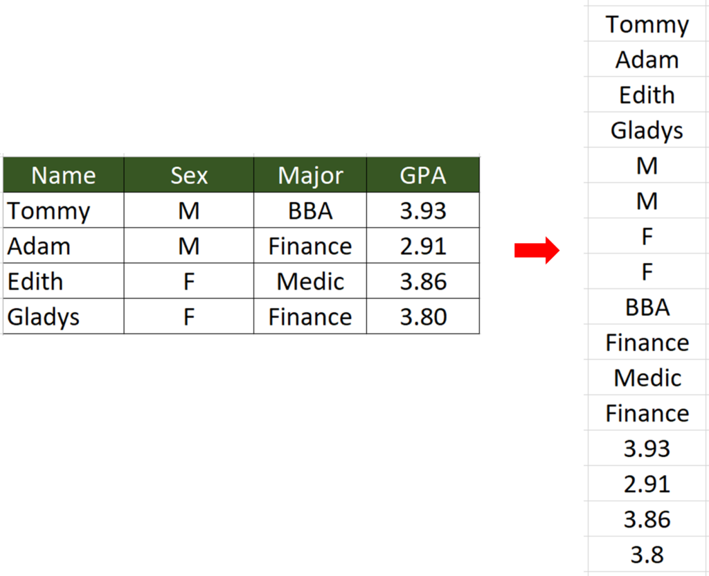
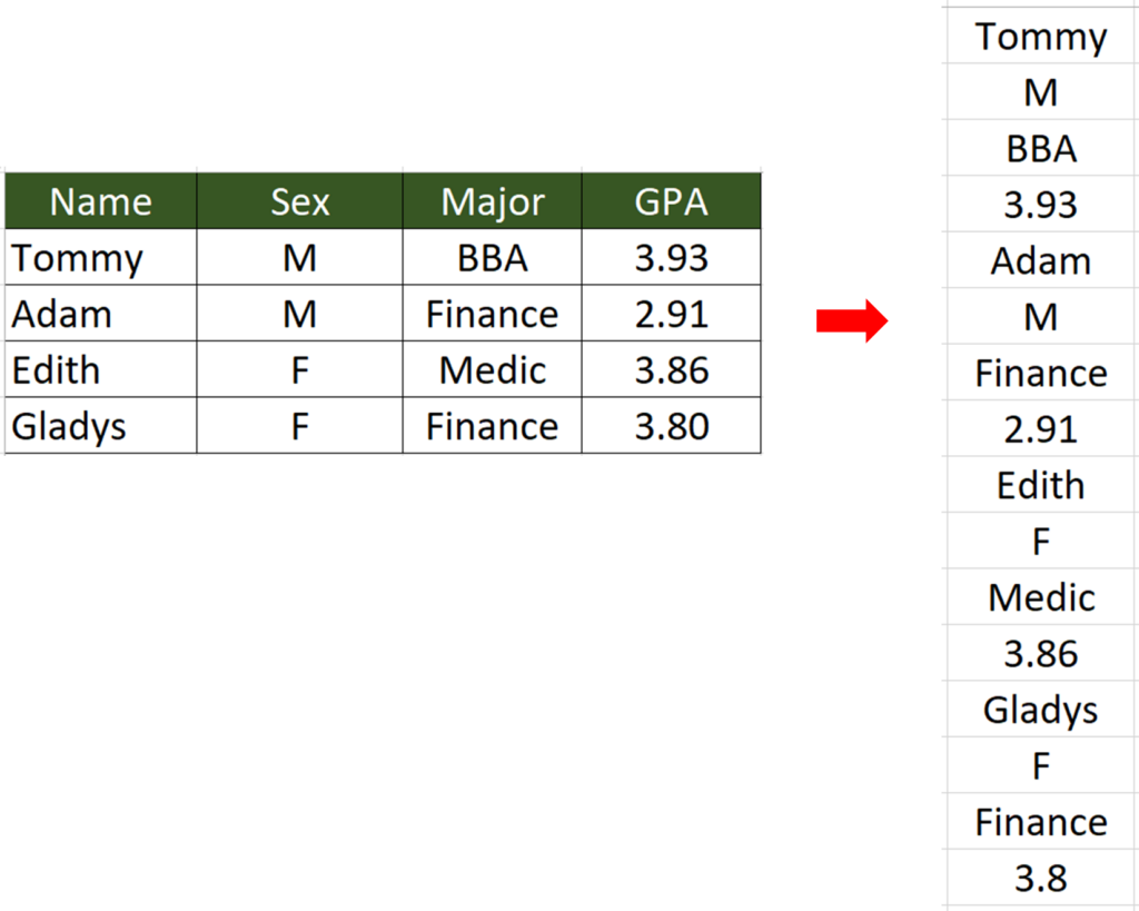
What we would like to do
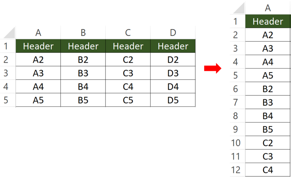
To stack multiple columns into one column, from top to bottom and then from left to right
You might also be interested in How to prevent duplicate entries in Excel?
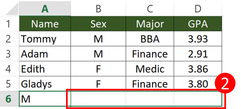
Step 1: Enter this formula right below the end of the first column
Formula
=the_first_cell_of_the_second_column
In the example, the first column ends at cell A5. So, I input the formula into cell A6.
It is such a neat formula, right?
I have seen people done this with a much complicated formula.
I would say
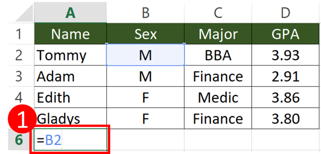
You may wonder why cell B2 instead of cell B1 is put here.
This is because I don’t want to include row 1 in my final results. If that is what you want, you can input B1 instead of B2.
Let me show you how the end result would look like if I have put B1 instead.
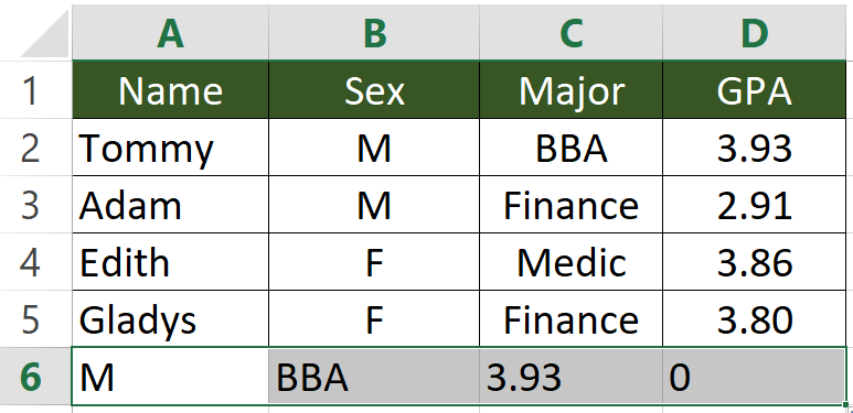
Step 2: Hover on the lower right corner of the cell and drag it until the last column
When you put your mouse pointer over the lower right edge of the cell, you will see a small black plus sign.
Click the black plus sign and drag it over to the last column (column D in this case) and don’t release your finger until you reach the last column.
This feature is called Autofill. It automatically fills in a series of cells for you.
When you do this, make sure you have selected the cell. Otherwise the small black plus sign won’t appear.
The table should look like this when you release the left mouse button.
Step 3: Hover on the lower right corner of the cell and drag it until the last row
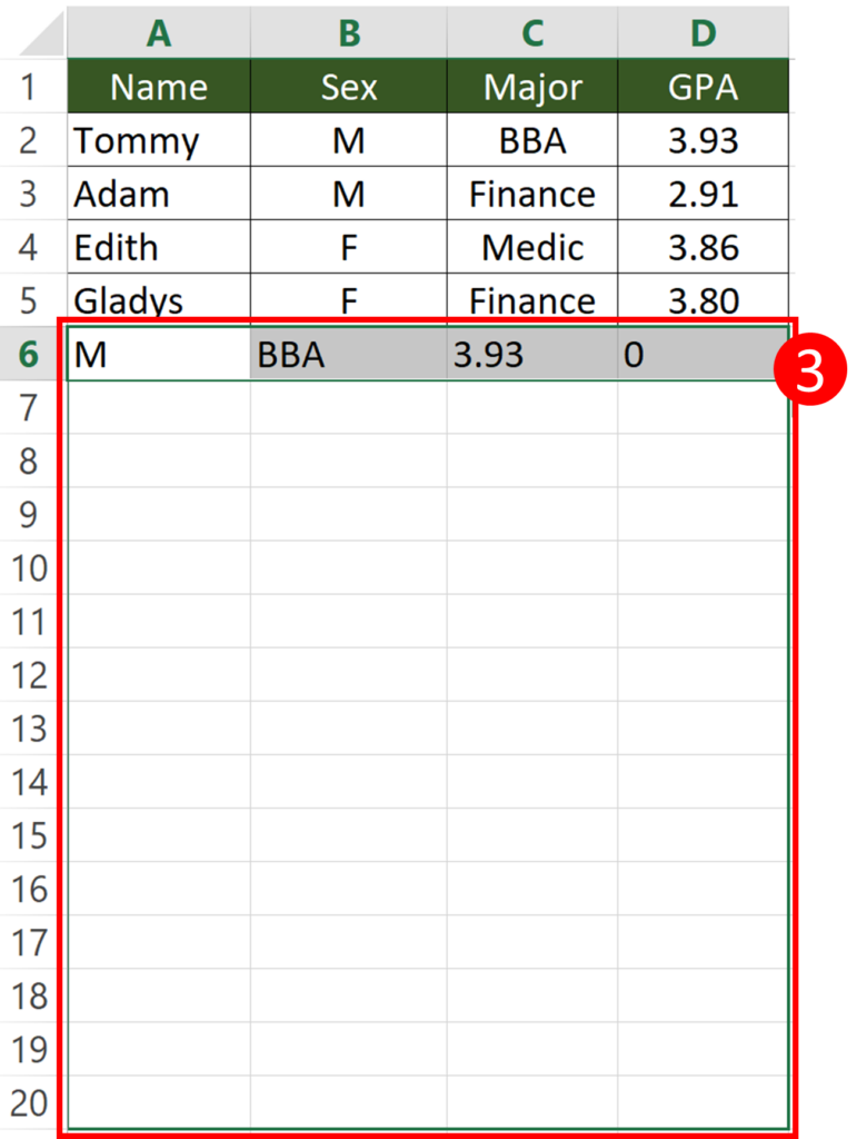
Step 3 is very similar to step 2.
Once again, we will need to make use of the Autofill feature in Excel.
The only thing that is different is that this time we are going to drag the small plus sign downwards.
In the previous step, we dragged the small plus sign rightwards until the last columns.
This time, we will need to drag the sign downwards until the last row.
You may wonder which row to drag until.
Usually, I just follow my heart. I will drag this down randomly and stop at a point where I think is right.
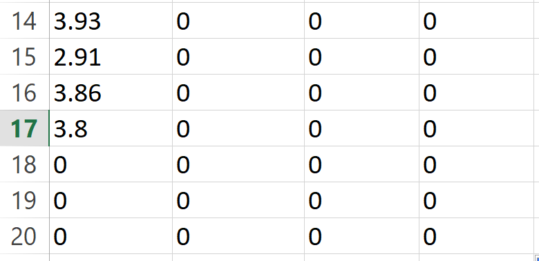
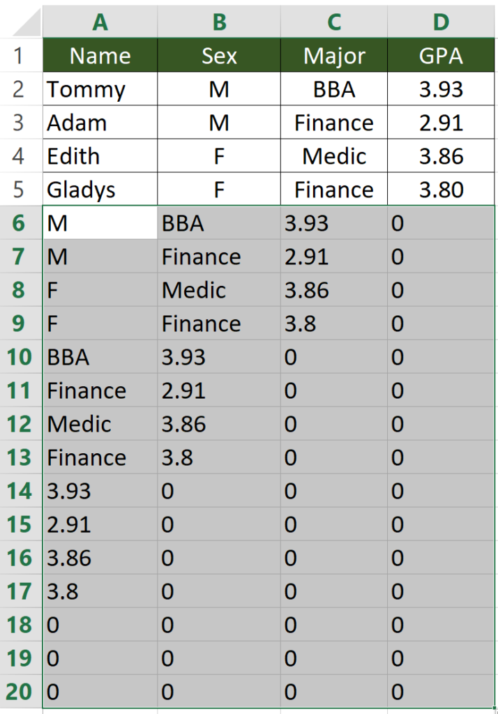
If I dragged more than I need, the extra rows will contain a “0”. I just delete them.
If you drag too much, you don’t need to worry for now. We will fix that later.
The table should look like this when you release the left mouse button.
Step 4: Copy and paste values

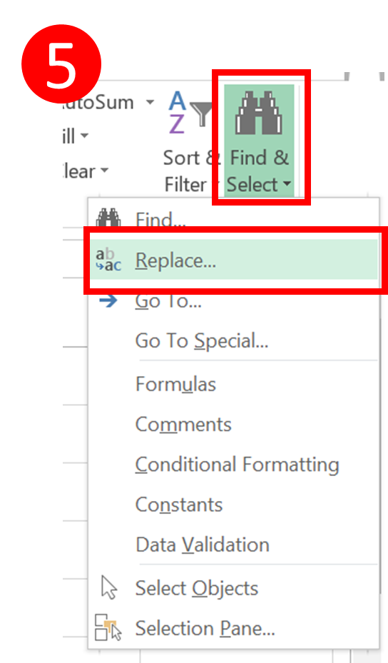
Step 5: “Home” > “Find & Select” > “Replace”
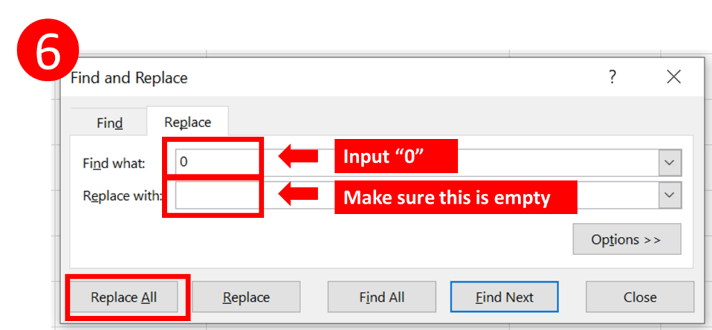
Step 6: Input “0” in “Find what” field > empty the “Replace with” field > Press “Replace All”
Here we will replace all “0” with nothing.
Make sure the “Replace with” field is empty. Not even space is allowed.
After pressing “Replace All”, you will see a pop up window telling you how many replacements have been made.
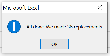
Then you can close the replace window by pressing Esc key.
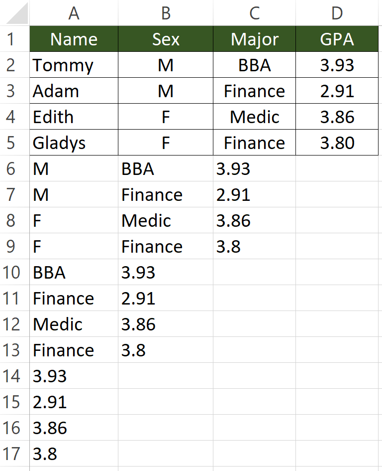
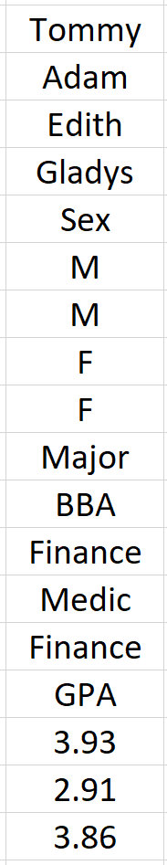
The table should look like this now. All we have to do is to delete the extra data.
In this case, cell B6 to cell B17 and cell C6 to C9 are redundant.
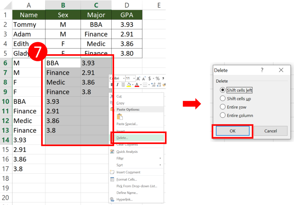
Step 7: Select the redundant cells and click the right mouse button > Press “Delete” > Press “OK”
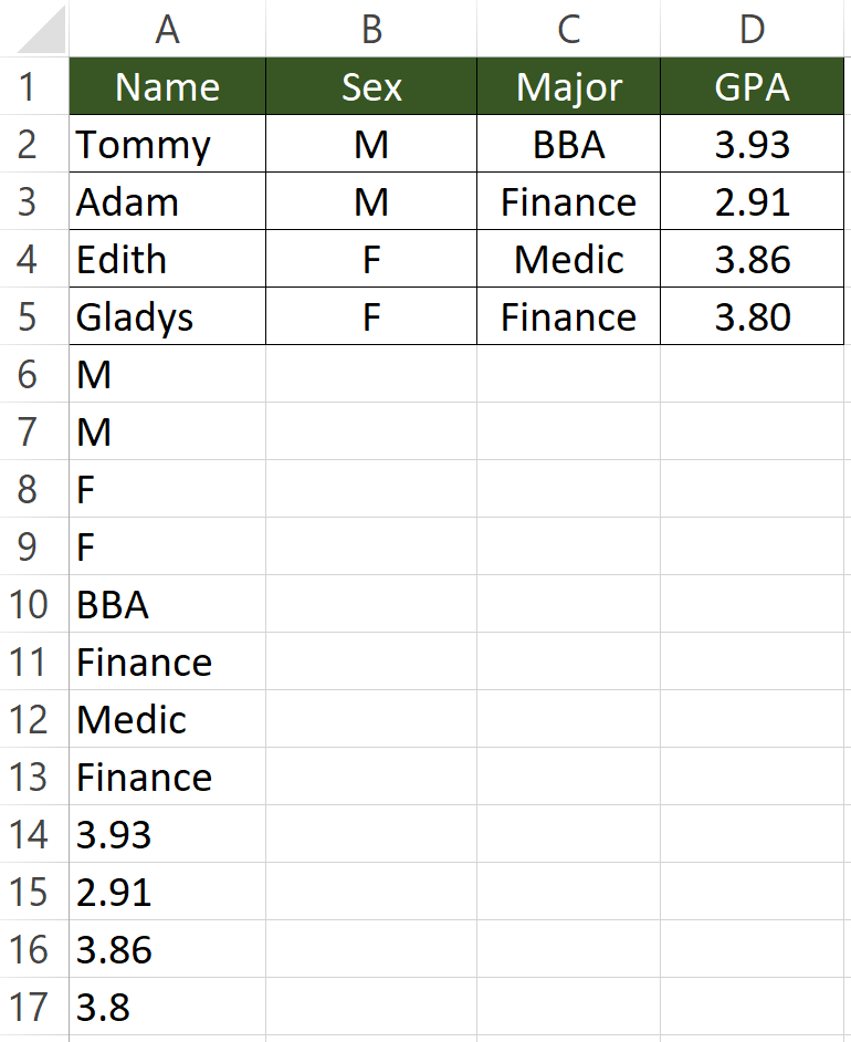
Result
You might also be interested in 6 Ways To Converting Text To Number Quickly In Excel
Stack Multiple Columns into One Column by formula (left to right)
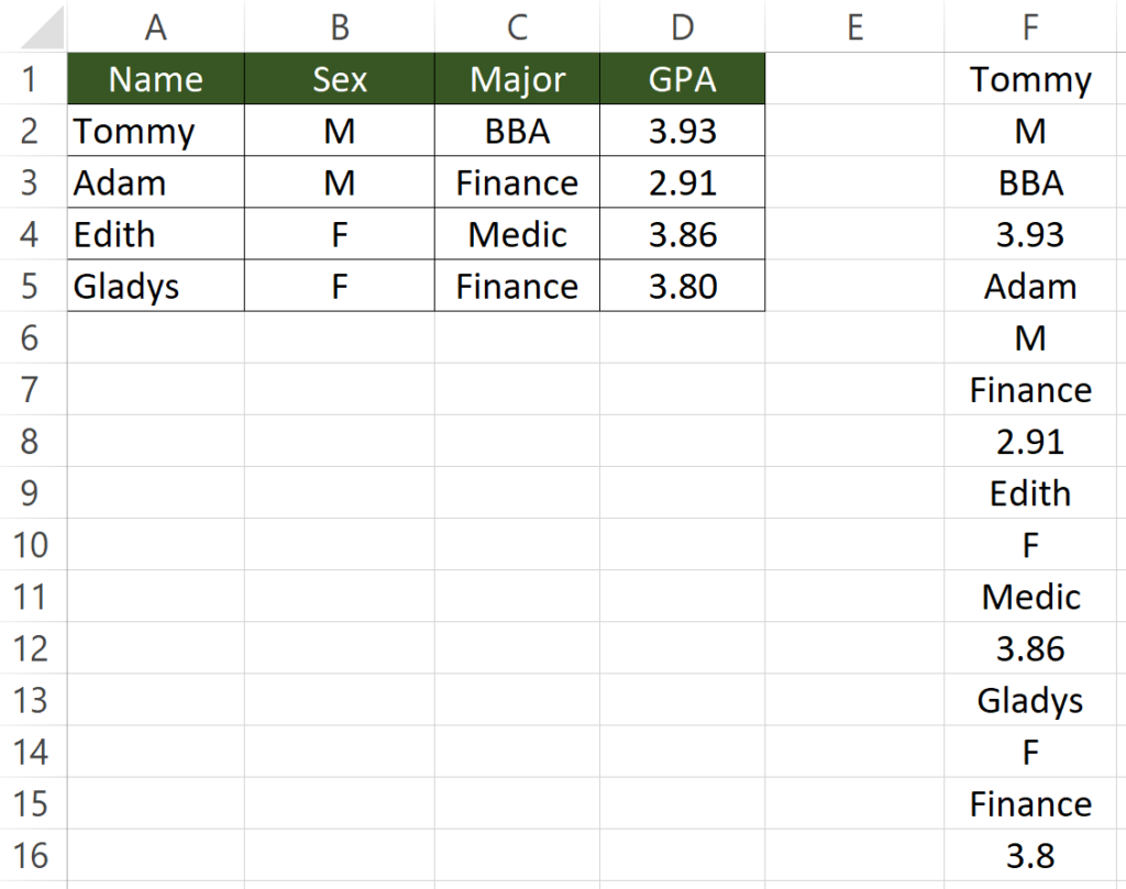
All we need is a formula.
Formula in Cell F1
=INDEX($A$2:$D$5,1+INT((ROW(A1)-1)/COLUMNS($A$2:$D$5)),MOD(ROW(A1)-1+COLUMNS($A$2:$D$5),COLUMNS($A$2:$D$5))+1)
How to use the formula
=INDEX(Original_table,1+INT((ROW(A1)-1)/COLUMNS(Original_table)),MOD(ROW(A1)-1+COLUMNS(Original_table),COLUMNS(Original_table))+1)
In the above example, the table starts from cell A2 and stop at cell D5. So we will put A2:D5 as the Cell_range. Make sure you lock the cell (Add dollar sign to each cell). The shortcut to lock cells is to press F4.
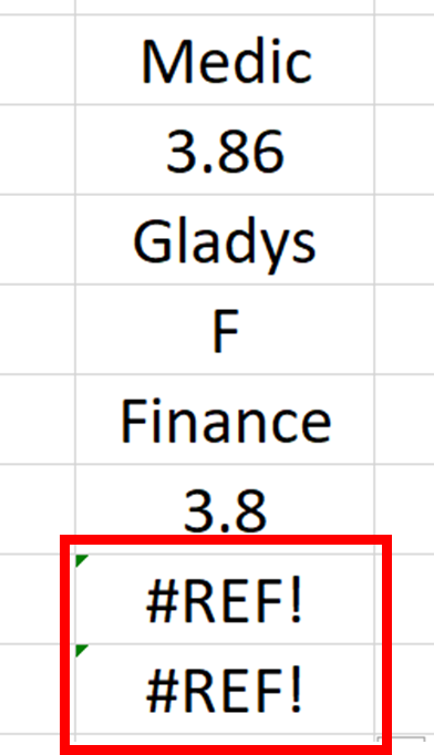
We are almost there.
Just make sure you got the formula in the first cell right. Then you can copy the cell down until you saw a #REF error.
The formula may seem a bit complicated at the first glance but it is not.
It doesn’t require much effort to edit the formula.
Stack Multiple Columns into One Column by VBA (left to right)
**Read How to Insert & Run VBA code in Excel – VBA101 if you forget how to insert VBA code in Excel.
Sub StackColumnIntoOne()
    Dim Tablerng, Destinationrng, Rng As Range

    'Get table range by inputbox
    Set Tablerng = Application.InputBox(Prompt:="Please select the table range", Type:=8)
    'Get destination range by inputbox
    Set Destinationrng = Application.InputBox(Prompt:="Please select the Destination cell", Type:=8)

    For Each Rng In Tablerng.Rows
            'Copy each cell inside the table
            Rng.Copy
            'Paste them into the destination column
            Destinationrng.Offset(RowIndex, 0).PasteSpecial Paste:=xlPasteAll, Transpose:=True
            RowIndex = RowIndex + Rng.Columns.Count
    Next

End Sub
What this VBA code does
This VBA code does the exact same thing as the Other VBA articles How to Check/Test if Sheets Exist in Excel? How To List All Worksheets Name In A Workbook How to Unpivot or Reverse Pivot in Excel You might also be interested in How To Remove Digits After Decimal In Excel? Hungry for more useful Excel tips like this? Subscribe to our newsletter to make sure you won’t miss out on any of our posts and get exclusive Excel tips!