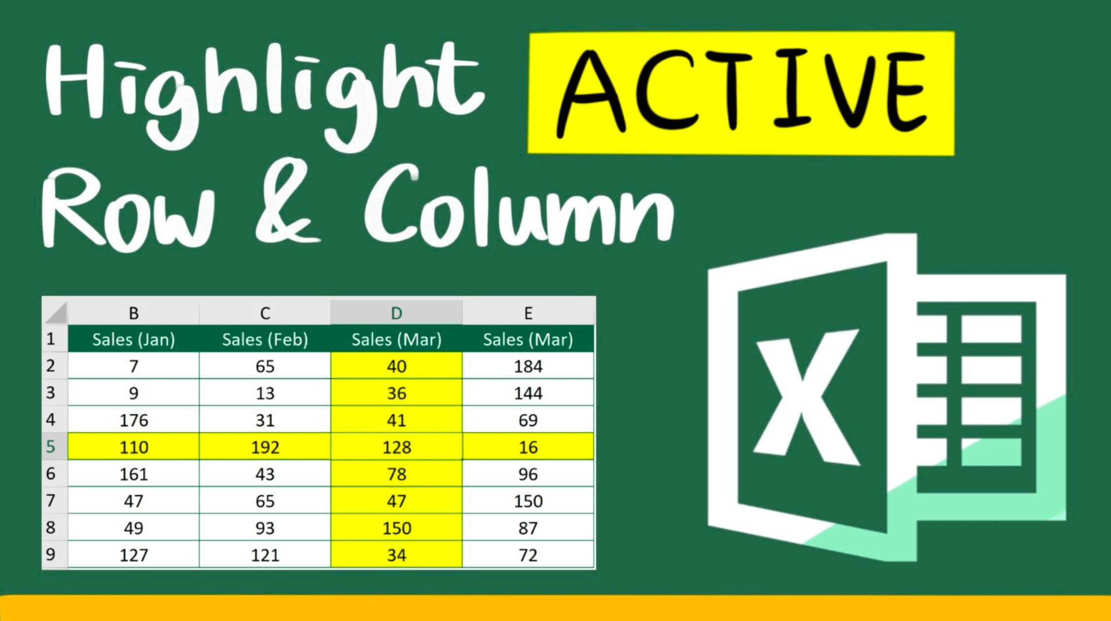
Sometimes you may have a big chunk of data in Excel. You may easily get lost when you are looking at the data. Do you know you can create a spotlight effect with a few steps?
In this article, I will show you how to highlight current row and column in Excel by changing the number format of cell. It comes especially handy when you are trying to show someone else your Excel spreadsheet.
When it comes to highlighting current row and column in Excel, many would have suggested using VBA. However, some of the Excel beginners might find it too demanding and refuse to learn VBA. Here I will provide you with an alternative.
You will be able to highlight current row and column in Excel without using VBA. All you need is a neat formula.
If you have the following questions, I suggest you reading this until the end.
- How to create spotlight effect in Excel?
- How to highlight current column and row in Excel?
- How to highlight active cell in Excel?
Example
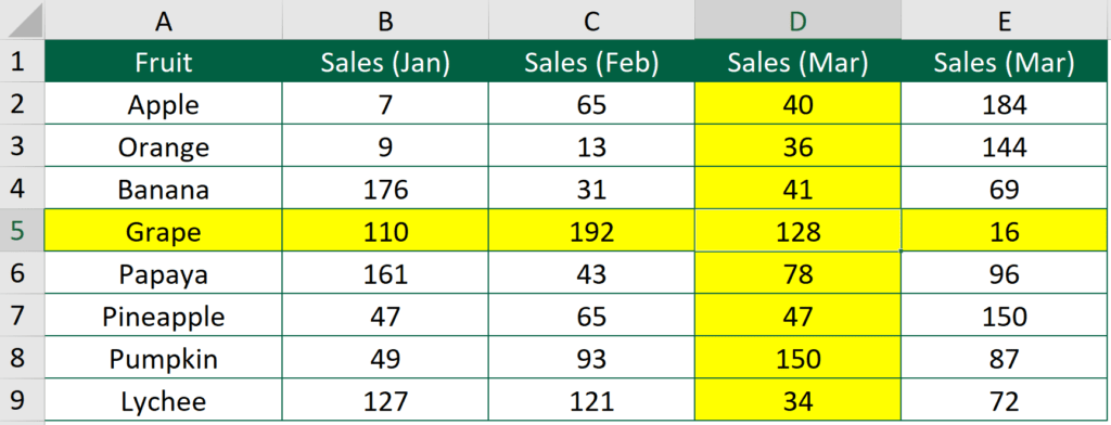
In the above example, the active cell is D5.
Column D and row 5 are highlighted in yellow.
What we would like to do
To highlight current row and column
You might also be interested in How to prevent duplicate entries in Excel?
Highlight current row and column in Excel by changing the number format
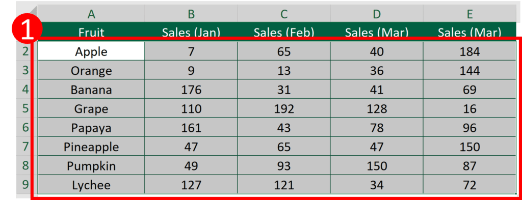
Step 1: Select the area to be highlighted
Make sure you only select the cell area that is necessary. Selection of extra area may lead to extra calculation effort, thus slowing your Excel file.
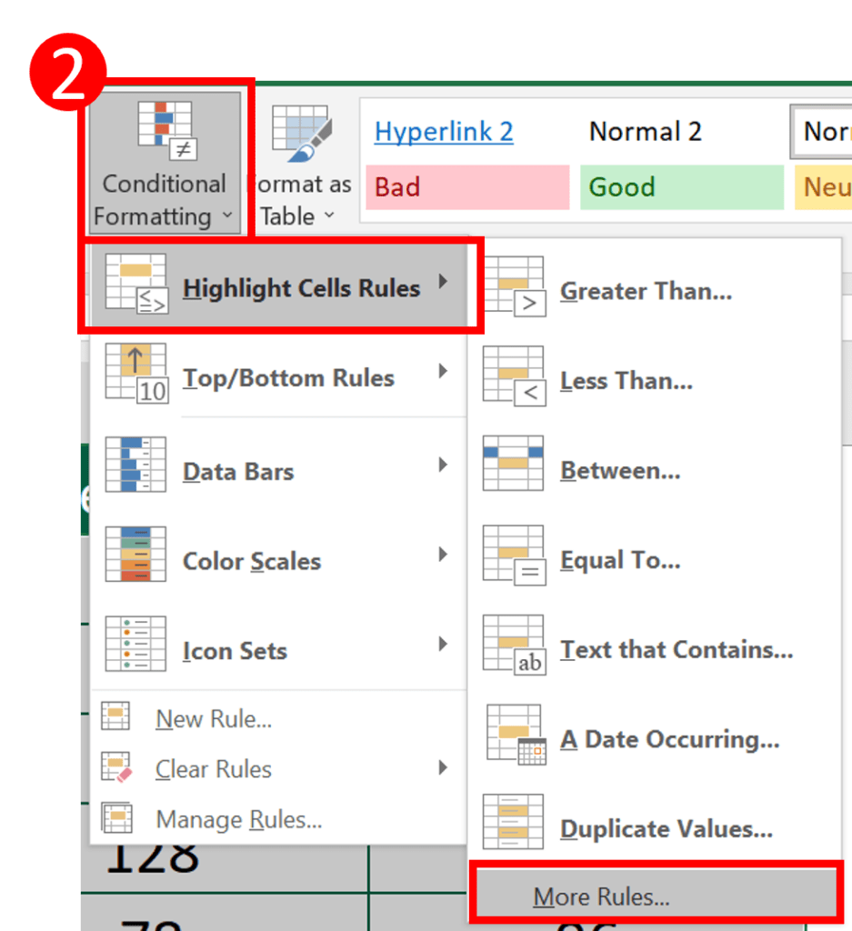
Step 2: Select Conditional Formatting>Highlight Cell Rules> More Rules
Usually the Highlight Cells Rules would have satisfied our need for conditional formatting. Yet this time we need something more dynamic and flexible.
Instead of selecting the normal rules, we are going to create rules of our own.
That’s why we need to select “More Rules”.
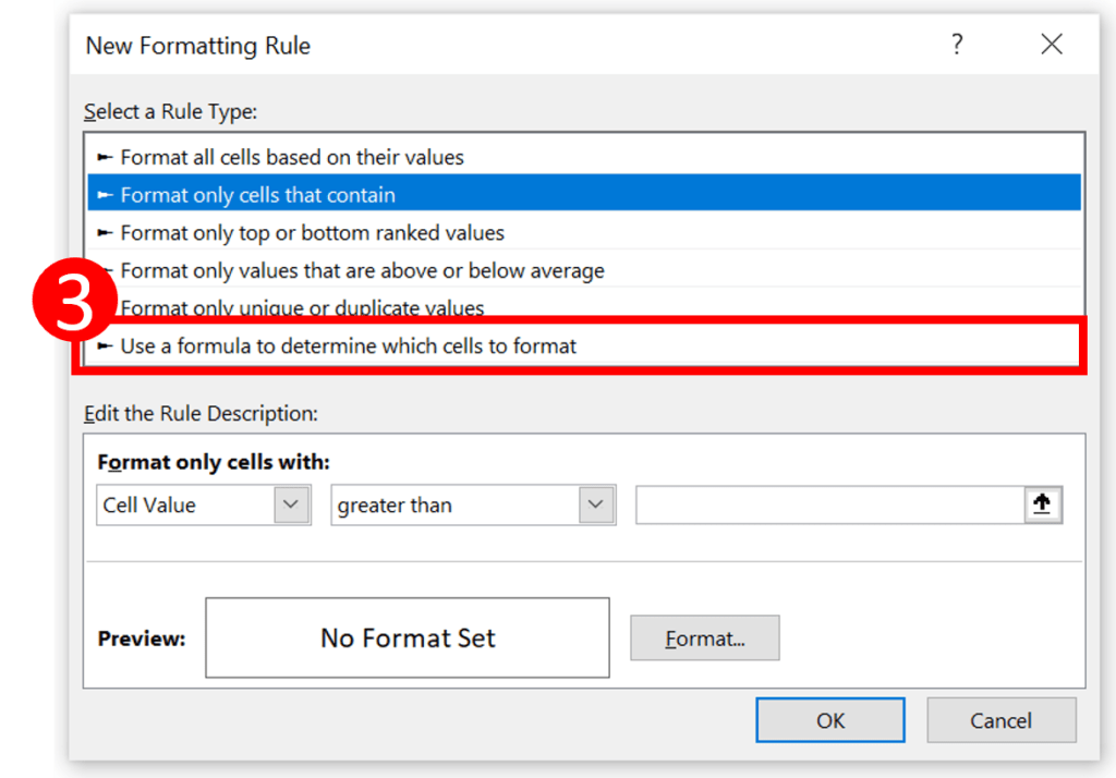
Step 3: Select “Use a formula to determine which cells to format”
I am aware that many of you do not have the experience of creating formula inside conditional formatting rules.
Don’t panic. We will do it together.
Step 4: Enter this formula in the “Format values where this formula is true” field and press “Format”
=OR(CELL("row")=ROW(),CELL("col")=COLUMN())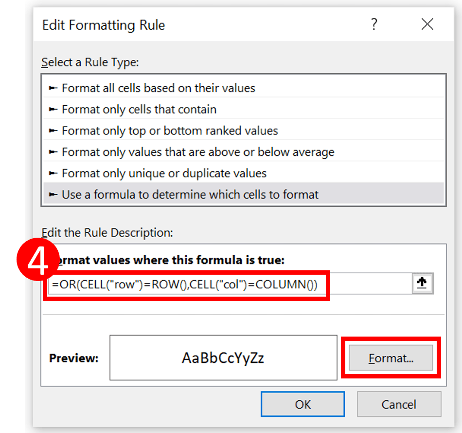
You might also be interested in Black-Scholes Option Pricing (Excel formula)
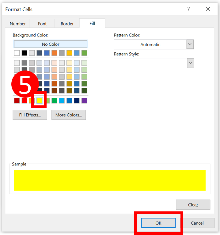
Step 5: Choose a style you like and press OK
I prefer the highlighted cell to have a yellow background so I can see it clearly.
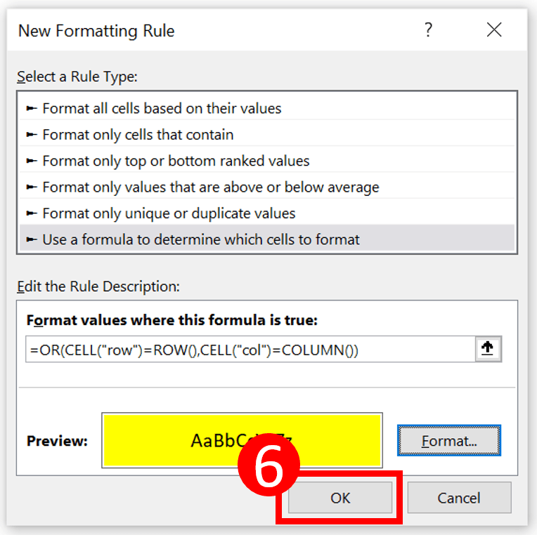
Step 6: Press OK
Step 7: Press F9
F9 is the shortcut of calculating all worksheets in all open workbooks.
Whenever you want the row and column of the active cell to be highlighted, you have to press F9.
The best part of this method is that it doesn’t require VBA. It doesn’t require you to modify the formula either.
Anyone who follows the step can do this.
You might also be interested in 5 Types of Graphs to Create with REPT function
Hungry for more useful Excel tips like this? Subscribe to our newsletter to make sure you won’t miss out on any of our posts and get exclusive Excel tips!