Inserting blank rows can be time consuming, especially when you have a large set of data. Inserting blank row every other row is however a frequently performed action. Is there any way to perform it efficiently? Yes! With the following tricks, you will no longer have to insert the blank rows one by one.
In this article, I will show you how to insert every other row or every nth row in Excel. I assure you this tutorial will save you lots of effort.
If you have the following questions, I suggest you reading this until the end.
- How to insert every other row or every nth row in Excel?
- How to insert blank row in bulk in Excel?
- How to insert blank row between every nth row in Excel?
You might also be interested in 5 Types of Graphs to Create with REPT function
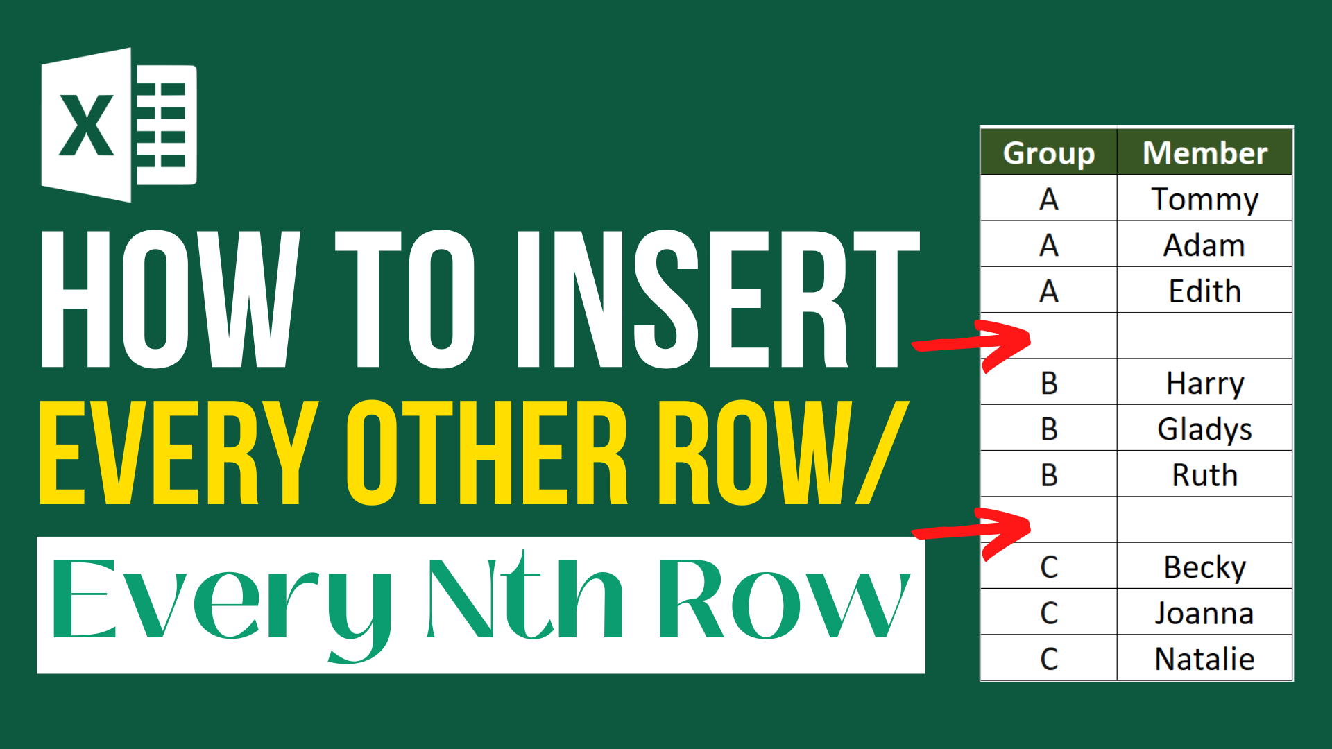
Insert every other row in Excel (Example 1)
In this sample, we are going to insert a blank row after each row. If you are looking for ways to insert every nth row, please jump to the next session.
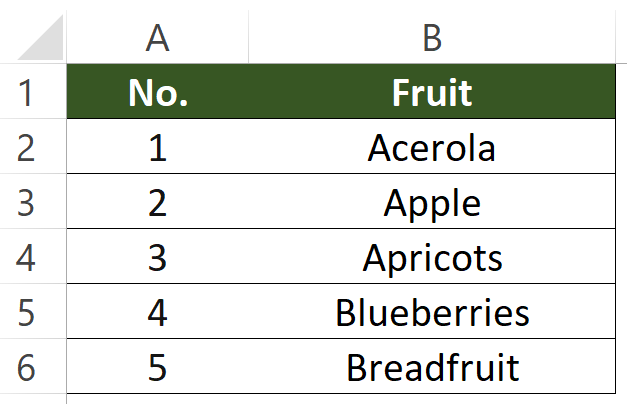
Step 1: Add serial number right next to the original column
You can enter the serial number manually or use the fill handle.
How to use the fill handle to enter serial number? Enter 1 in a cell > press Ctrl and drag the little + handle until you see the number you want > release your finger.
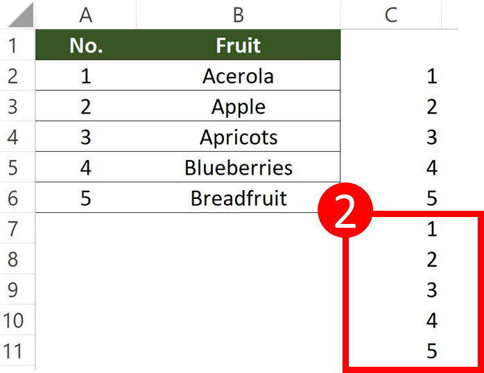
Here I drag the handle until I saw 5.
Here we are trying to make an auxiliary column.
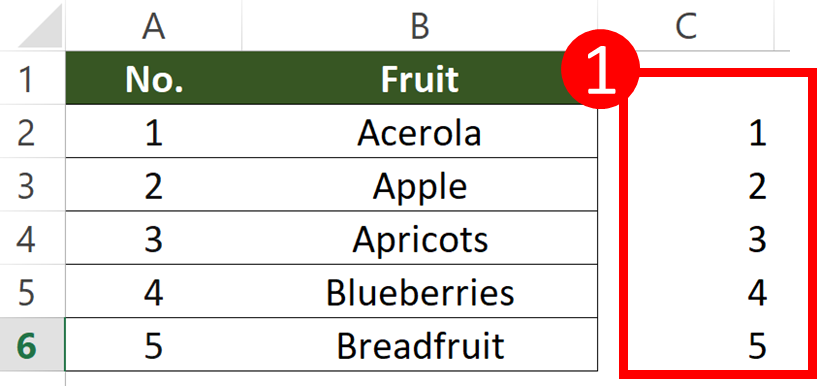
Step 2: Copy the set of serial number and paste it right below
Just now we have enter 1 to 5 into column C. Now we will need to copy those number and paste it right below the original set of serial number.
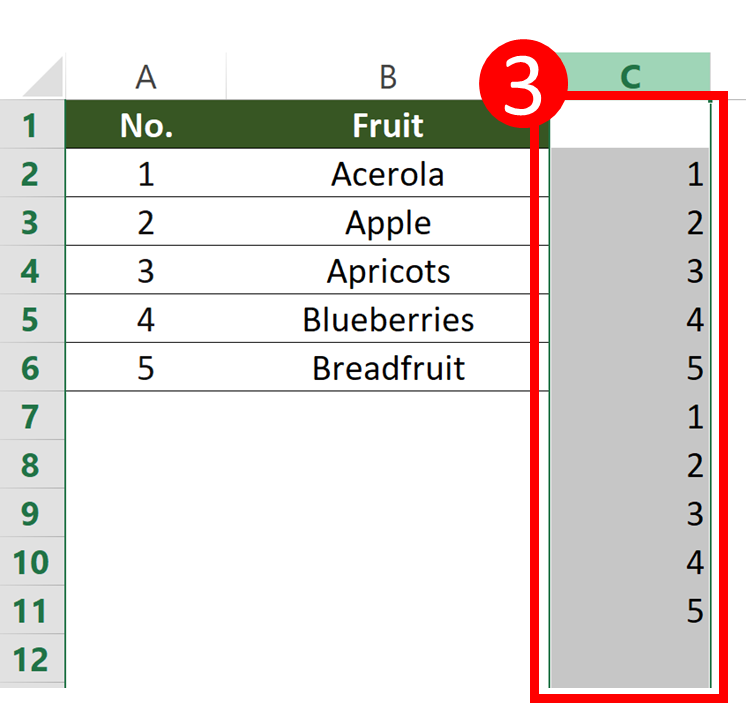
Step 3: Select the column that contains serial number
Now you will need to select the column that we just put in serial number.
You can do that by pressing the column header or pressing CTRL + SPACE.
You might also be interested in Edit The Same Cell In Multiple Excel Sheets
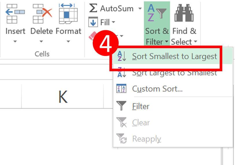
Step 4: Select “Home”> “Sort & Filter” >”Sort Smallest to Largest”
“Sort & Filter” is in the Editing group.
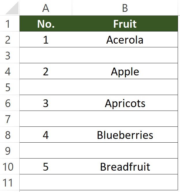
Result
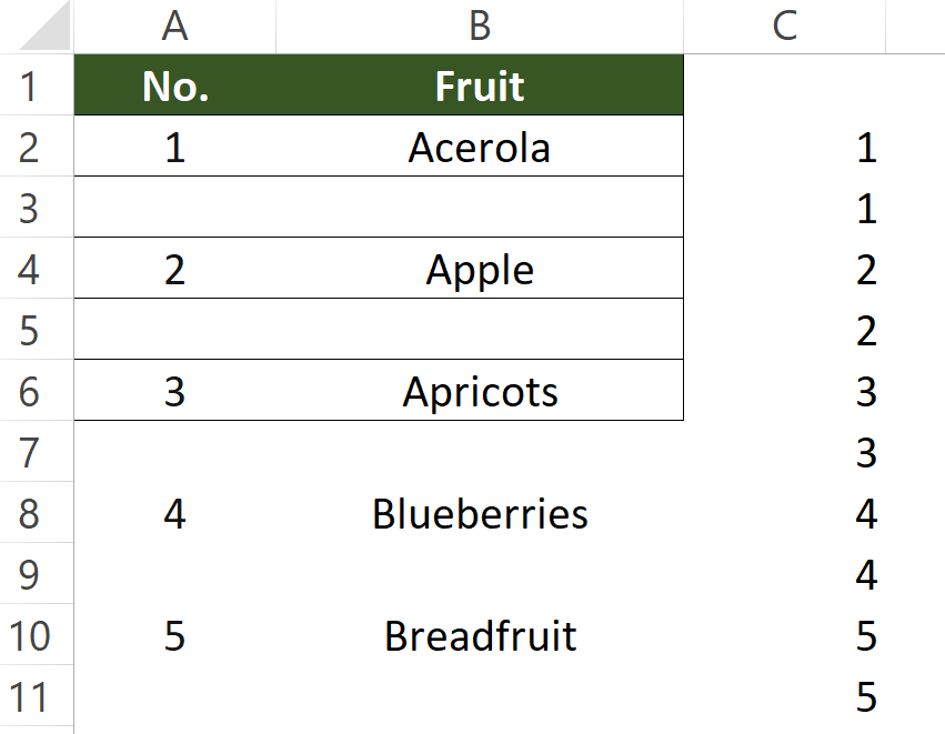
After this, you can delete the auxiliary column.
You might also be interested in 6 Ways To Converting Text To Number Quickly In Excel
Insert every nth row in Excel (Example 2)
In this example, we are going to insert a blank row every 3 rows. The result should look like this.


Step 1: Insert a column next to the original column and apply this formula
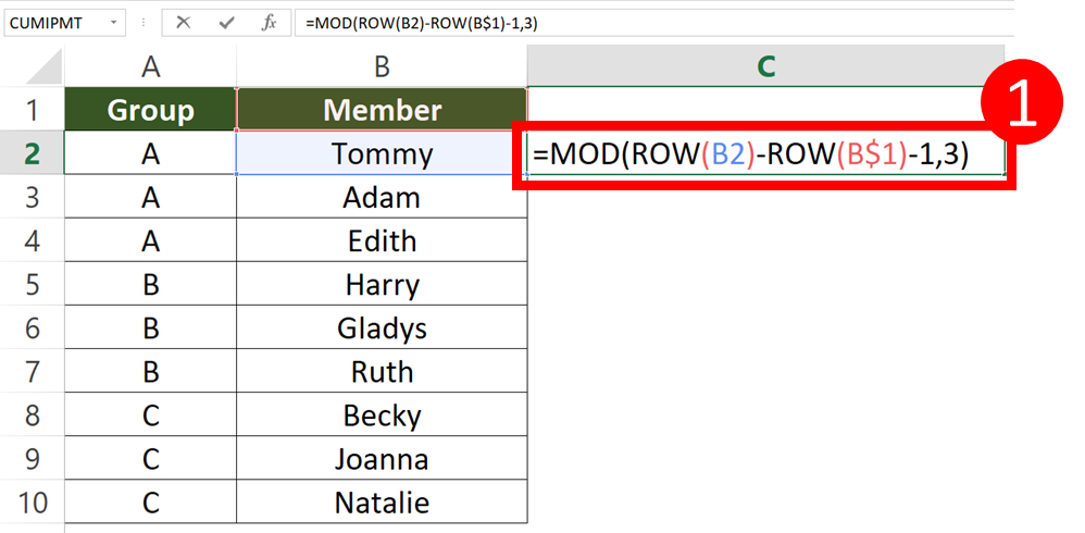
=MOD(ROW(B2)-ROW(B$1)-1,3)
How to use the formula
=MOD(ROW(First_cell_of_the_column)-ROW(Cell_above_the_first_cell_of_the_column)-1,Number)
In this example,
Cell_above_the_first_cell_of_the_column = B1 (The cell contains the text “Member”)
First_cell_of_the_column = B2 (The cell contains the text “Tommy”)
Number = Every Nth row = (For instance, put a 6 here if you want to insert blank row every 6 row)
Make sure you lock the cell in the formula.
Since I would like to insert a blank row every 3 row, I will put a 3 here.
Step 2: Copy the formula down
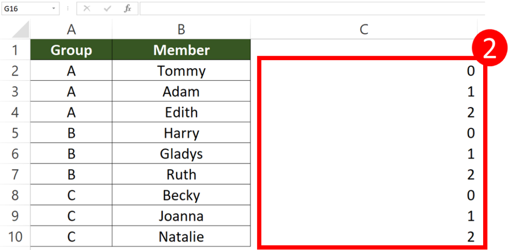
You can achieve that by 2 easy ways.
- Copy and paste formula (Ctrl+C, Ctrl+Alt F OK)
- Auto fill (Double click the lower right corner of the first cell)
You might also be interested in How to Select Cells with Colour (3 ways + VBA)
Step 3: Select the auxiliary column
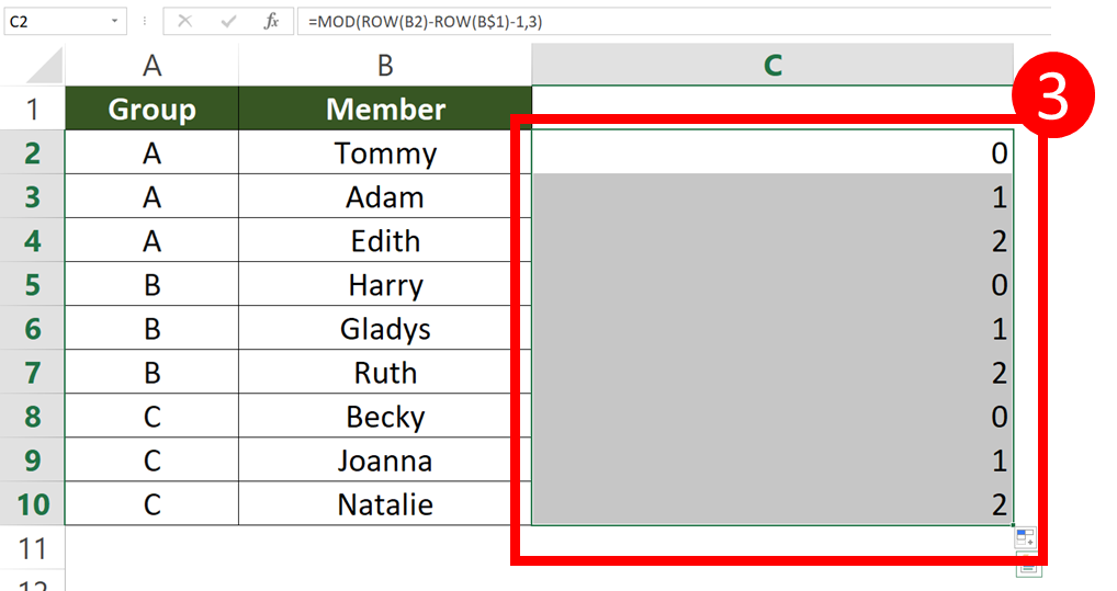
Step 4: Press Ctrl + C, then press Ctrl + Alt + V, V
Ctrl C is the shortcut to copy. Ctrl + Alt + V is the shortcut to open the paste special window. The remaining V is the shortcut to select paste values only.
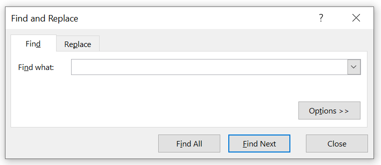
Step 5: Press Ctrl + F
If you unselect the cells after previous action, select the cells again.
This should trigger the “Find and Replace” window.
Step 6 & 7: Put “0” in the “Find What” box and press “Find All”
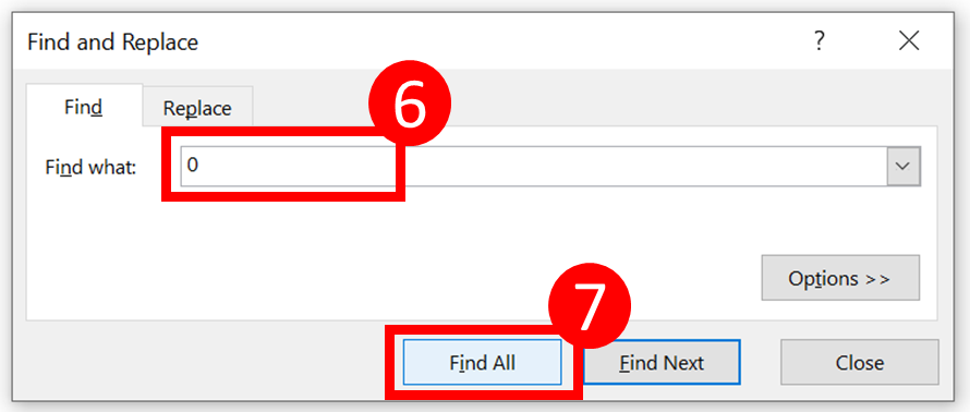
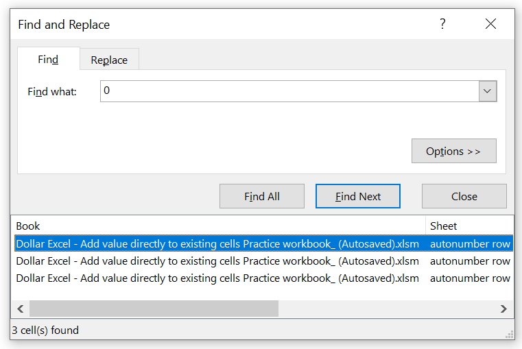
The window should turn into this after step 7.
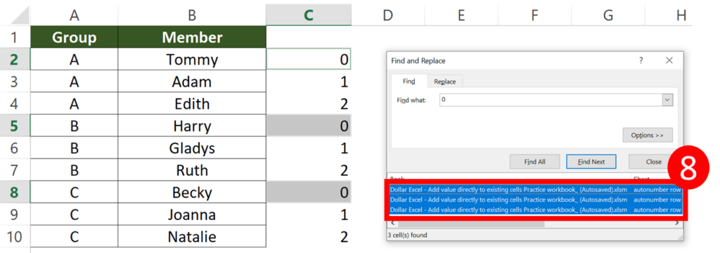
Step 8: Press Ctrl +A
Ctrl + A is the shortcut to select all.
When you press Ctrl + A, you will see that every 0 within the range you just selected has become the new selection.
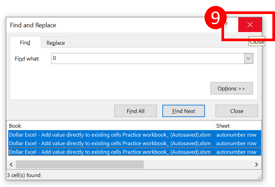
Step 9: Close the window
Step 10: Press Ctrl Shift +
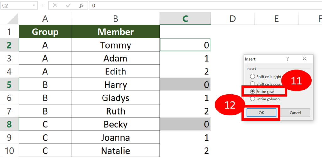
Step 11 & 12: Select “Entire row” and press “OK”
Result

You can delete the first blank row and the auxiliary column if you don’t need it anymore.
You might also be interested in How To Remove Digits After Decimal In Excel?
Then, you can repeat the step 4 to step 6 in the above tutorial.
Hungry for more useful Excel tips like this? Subscribe to our newsletter to make sure you won’t miss out on any of our posts and get exclusive Excel tips!