


Numbering rows is one of the actions we perform in Excel on a daily basis. It will definitely save us some time if the action can be automated. Some may suggest copy and paste. However, mistake may happen if we fail to pay enough attention.
In this article, I will show you how to autonumber rows and skips blank rows. Since the number is produced by a formula instead of an exact number, it will change into the correct value every time the list changes. You no longer need to worry about the if the number is in the right order.
If you have the following questions, I suggest you reading this until the end.
- How to autonumber rows in Excel?
- How to autonumber rows and skip rows that are blank in Excel?
- How to number row in a way that it will change when there is change in row in Excel?
- How to make sure row number is in the right order in Excel?
You might also be interested in How to get value from every nth row?
Example
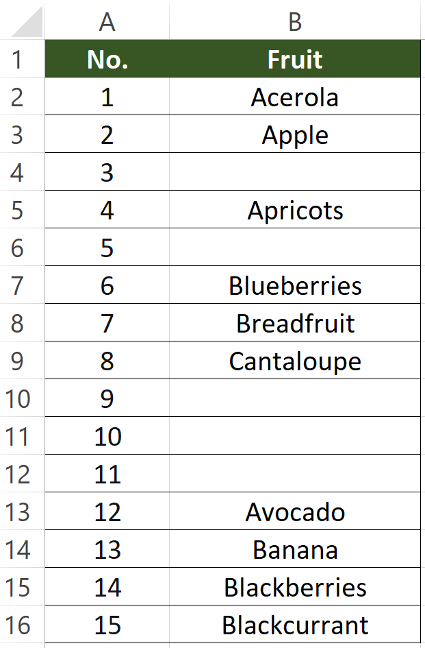
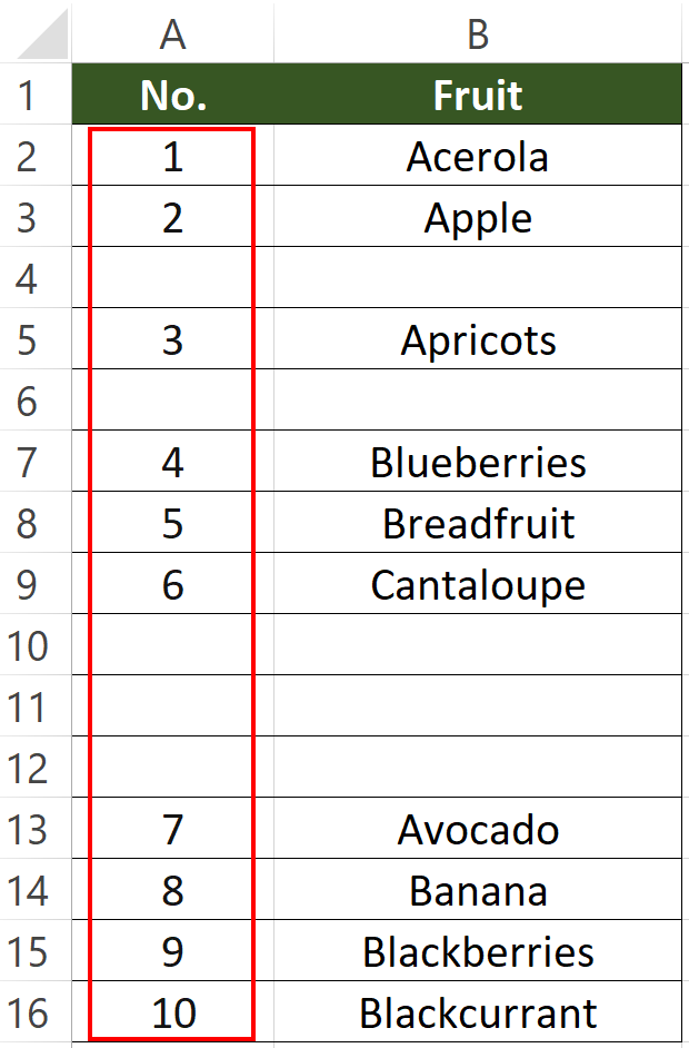
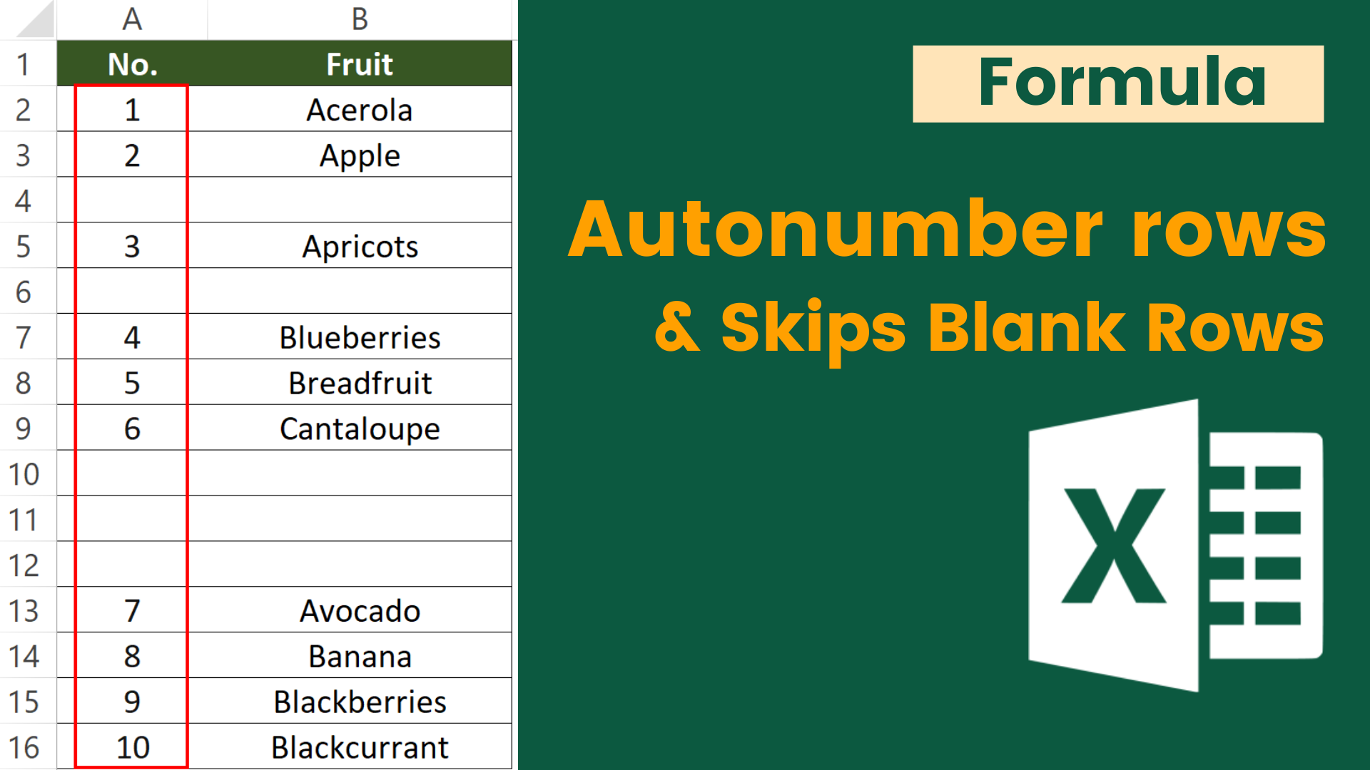
In the normal numbering example, the number next to “Apricots” is 4. In another example, the number next to “Apricots” is 3. This is the result we would like to achieve.
What we would like to do
To autonumber rows and skips blank rows
You might also be interested in How to prevent duplicate entries in Excel?
Autonumber rows and skips blank rows by formula
Formula in cell A2
=IF(B2<>"",COUNTA($B$2:B2),"")
For the remaining cells, just copy the formula down.
How to use the formula
=IF(First_cell_of_source_list<>"",COUNTA(First_cell_of_source_list(lock row and column):First_cell_of_source_list),"")
In the sample sheet, the first cell in the source list is cell B2.
“Why is it not cell B1?”
This is because we only count the value in the list but not the column header.
How does this formula work
COUNTA(First_cell_of_source_list(lock row and column):First_cell_of_source_list)
COUNTA function allows us to count the number of cells in a range that are not empty.
Here we are using COUNTA to count the number of non-empty cells between the corresponding cell (here it means the cell next to the cell with formula) and the first cell.
Take cell A5 as an example.
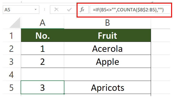
COUNTA functions counts the number of non-empty cells between the corresponding cell (B5) and the first cell in the list (B2). Let’s count it by hand. The number is 3 since there are three non-empty cells (B2, B3 and B5) in the specified range.
=IF(First_cell_of_source_list<>"",COUNTA(First_cell_of_source_list(lock row and column):First_cell_of_source_list),"")
IF function allows us to check whether certain conditions are met.
Here IF function help us check whether the corresponding cell is empty. It will only allows COUNTA function to perform if the cell is not empty. If the corresponding cell is blank, the cell will return blank.
You might also be interested in How to Merge Cells Across Multiple Rows/Columns.
Hungry for more useful Excel tips like this? Subscribe to our newsletter to make sure you won’t miss out on any of our posts and get exclusive Excel tips!