Background
Have you heard of a function called UNIQUE()? As its name suggests, the Excel UNIQUE function extracts a dynamic array of unique values from a range or array. A big applause to Microsoft!
When you search online for a function to get unique values, the top results urge you to give the UNIQUE function a shot.
However, very likely you will find the UNIQUE function missing. This is because currently UNIQUE function is only available to Excel 365 users. For Excel users of earlier version, you won’t find UNIQUE function available in Excel. Unless you switch to Excel 365 version, you won’t be able to activate UNIQUE function.
If you wish to get unique value without using any formula, I suggest you take a look at this How to get unique values in Excel? (6 ways).
Do you have the following questions?
- Excel Unique function alternative
- How to get unique values without unique version?
- How to get unique values in Excel?
- Get unique values Excel formula
What can Excel users of other version do if they want to get unique values from a list?
In this article, I will show you how to extract unique values from Excel list without using Unique function. You can either use a standard formula or an array formula. You will find perfect substitute for Unique function in Excel.
Sample Workbook
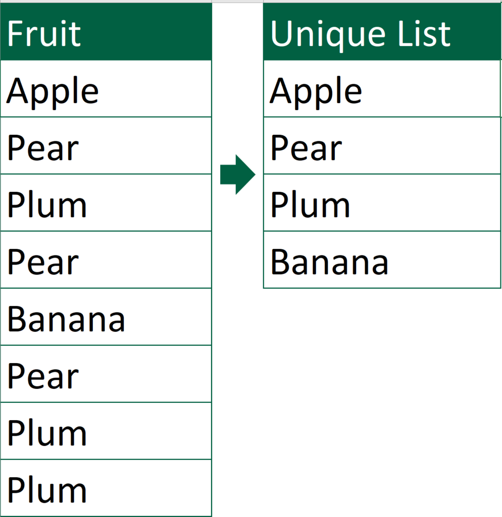
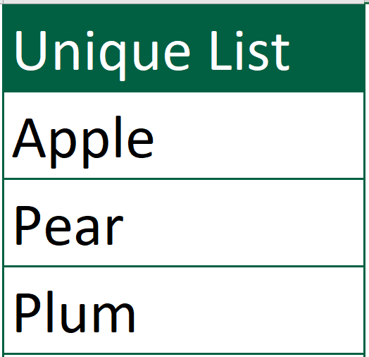
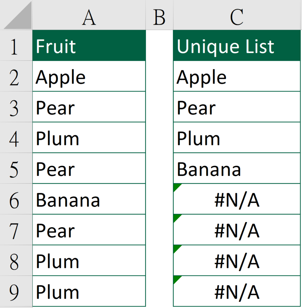
What we would like to achieve
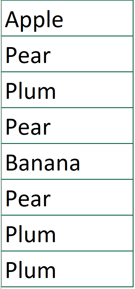
To extract unique list of values from the “Fruit” list
Download the workbook to practice it by yourself!
Press the download button!

Get Unique Values Without Unique function With Standard Formula
First, I will show you how to extract unique values from excel column using formula without array.
I understand that array formula can be a bit difficult for Excel beginners.
Here is the formula without array.
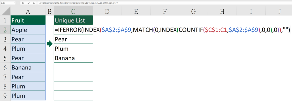
Formula of Cell C2
=IFERROR(INDEX($A$2:$A$9,MATCH(0,INDEX(COUNTIF($C$1:C1,$A$2:$A$9),0,0),0)),"")
Dollar Excel syntax
=IFERROR(INDEX(Original list, MATCH(0,INDEX(COUNTIF(Top cell of unique list column to itself, Original list),0,0),0)),"")
Things to be aware of
- Those highlighted in red means that you may need to change the reference
- Make sure the list start at row 2
- Make sure you don’t change any reference type
- Make sure the top cell of the unique list column doesn’t equal to other cell in the unique list
Get Unique Values Without Unique function With Array Formula
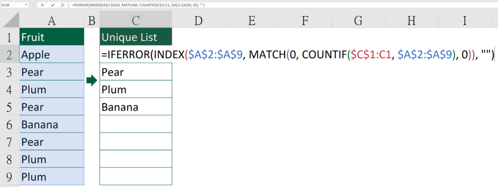
Formula of Cell C2
=IFERROR(INDEX($A$2:$A$9, MATCH(0, COUNTIF($C$1:C1, $A$2:$A$9), 0)), "")
Dollar Excel syntax
=IFERROR(INDEX(Original list, MATCH(0,COUNTIF(Top cell of unique list column to itself, Original list again),0),1),This is just an error handler to turn error value into zero)
Things to be aware of
- Those highlighted in red means that you may need to change the reference
- Make sure the list has a top cell
- Press Ctrl Shift Enter when finish editing the formula
- Make sure you don’t change any reference type
- Make sure the top cell of the unique list column doesn’t equal to other cell in the unique list
Explanation
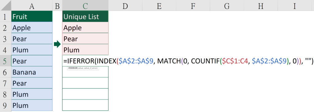
Formula of Cell C5
=IFERROR(INDEX($A$2:$A$9, MATCH(0, COUNTIF($C$1:C4, $A$2:$A$9), 0)), "")
Let’s dig deep into the array formula of extracting unique values.
To help you better understand the formula, I will explain each part of the formula according to the handling order.
This time we choose Cell C5 as the investigation object since you will be able to understand more with cell C5.
Part 1
COUNTIF($C$1:C1,$A$2:$A$9)
$C$1:C4 refers to “Unique List”, “Apple”, “Pear”, “Plum”
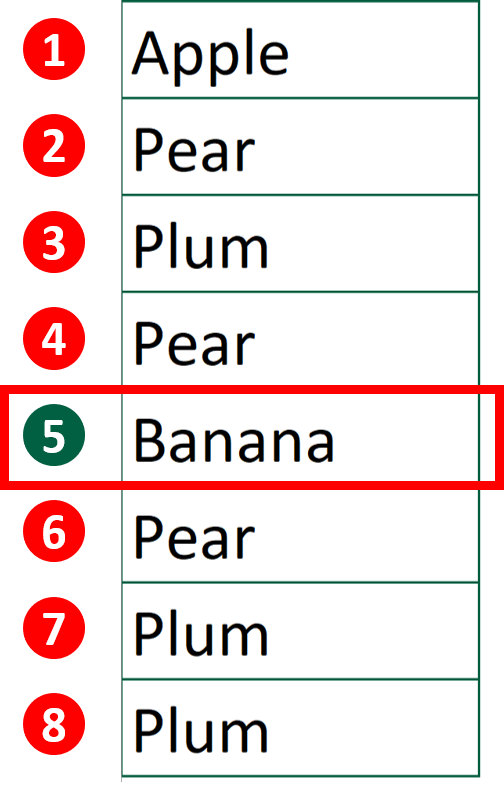
$A$2:$A$9 refers to “Apple”, “Pear”, “Plum”, “Pear”, “Banana”, “Pear”, “Plum”, “Plum”
COUNTIF function count cells that match certain criteria.
Here it counts the number of times $A$2:$A$9 appear in $C$1:C4.
Only “Banana” isn’t in the range $C$1:C4. It’s in Cell C5 instead.
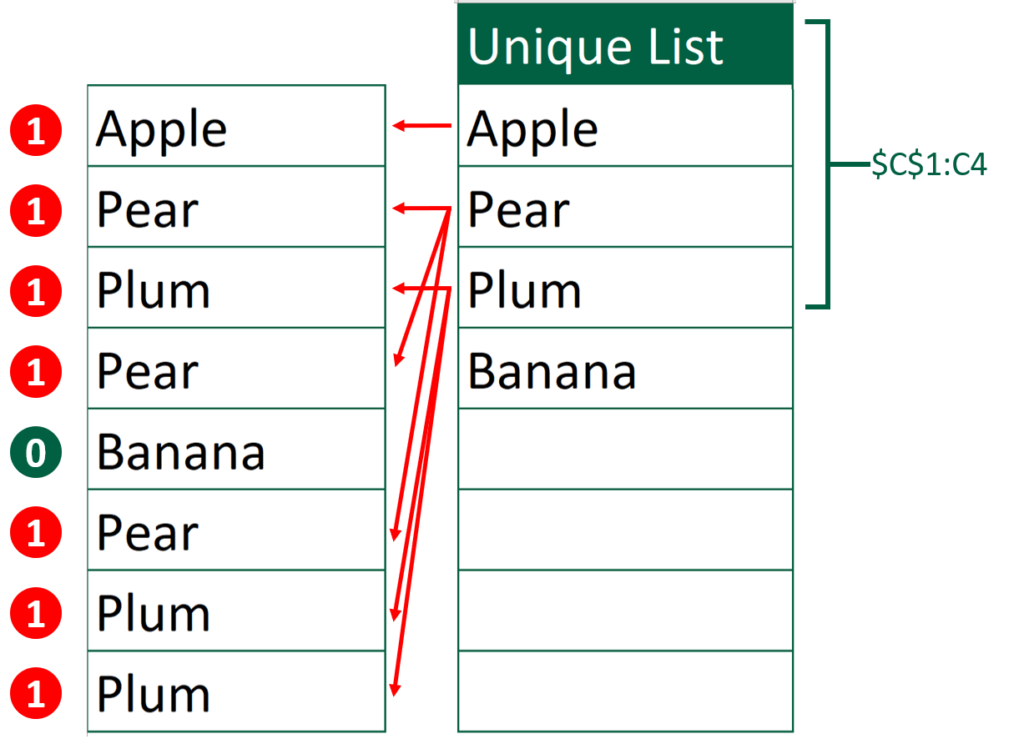
The result is {1, 1, 1, 1, 0, 1, 1, 1}.
Part 2
MATCH(0, COUNTIF($C$1:C4, $A$2:$A$9), 0)
After replacing COUNTIF($C$1:C4, $A$2:$A$9), we get this instead.
MATCH(0, {1, 1, 1, 1, 0, 1, 1, 1}, 0)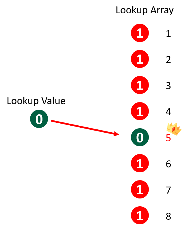
MATCH function returns the position of the matched value within an array.
Here the position of “0” in the lookup array is “5” so it will return a “5”.
Part 3
INDEX($A$2:$A$9, MATCH(0, COUNTIF($C$1:C4, $A$2:$A$9), 0))
After replacing above results, we get this instead.
INDEX($A$2:$A$9, 5)
INDEX function returns the nth item in an array.
Here we would like to return the 5th item in the $A$2:$A$9.
The result is “Banana”.
Part 4
IFERROR(INDEX($A$2:$A$9, MATCH(0, COUNTIF($C$1:C4, $A$2:$A$9), 0)), "")
After replacing above results, we get this instead.
IFERROR("Banana", "")IFERROR returns a specified value if it detects an error.
Here we set the specified value as blank.
Without the error-handling function, the result would appear as below.
Since we don’t have any error in the formula, it will return the original value, which is “Banana”.
If unique function is not available in Excel, I highly recommend you to try these two formula.
Do you find this article helpful? Subscribe to our newsletter to get exclusive Excel tips!