In this article, I will show you how to delete rows if cell in certain column is blank. It doesn’t matter if your workbook contains hundreds of worksheets.
Very often we will need to delete rows if cells in certain column does not contain any value. This may happens a lot when we have to break a large table into several small table. The deletion could have easily cost us a few hours.
If you have the following questions, I suggest reading this until the end.
- How to delete rows if cell in certain column is blank in Excel?
- How to delete every row that does not contain a value in certain column in Excel?
- How to delete rows if cells in empty in certain column?
You might also be interested in Excel Split Long Text into Short Cell Without Splitting Word.
Example
To help you better understand how to delete row if cells in certain column contains no content, I have created an example below.
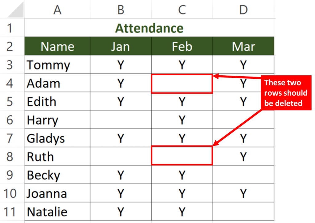
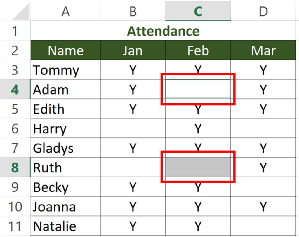
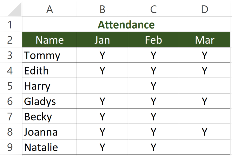
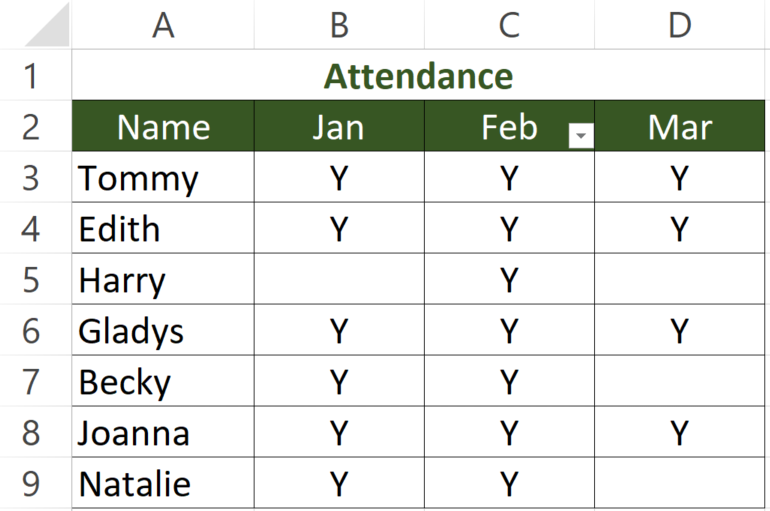
This is a table of attendance. Attendance of each student is indicated by a letter “Y”.
We would like to make a table that includes only people who attended the February session.
In other words, Adam and Ruth should be excluded from the list.
What we would like to do
To delete rows if cells in column C is blank
You might also be interested in How to prevent duplicate entries in Excel?
Delete Row if column is Blank by “Go To Special”
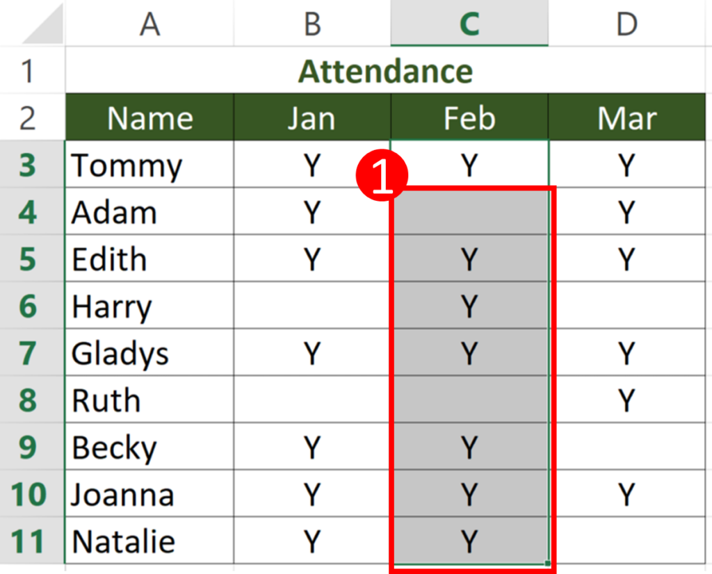
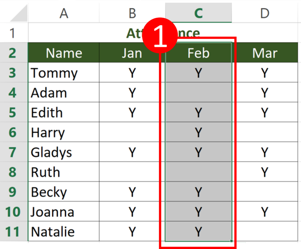
Step 1: Select the cell range
Since column C will help me identify which row to be deleted, I selected cells in column C.
If you would like to delete rows which cells in column D is blank, then you should select column D.
Here I didn’t select the whole column. You can select the whole column if there is nothing under the table.
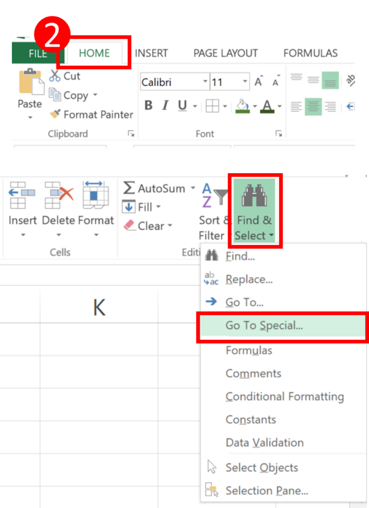
Step 2: Select “Home” > “Find & Select” > “Go To Special”
“Find & Select” is usually at the rightmost part of the ribbon.
After you pressed “Find & Select”, you should see “Go To Special”.
In case you need it, the shortcut to open “Go To Special” window is Ctrl + G, Alt + S.
When you pressed Ctrl + G, you triggered “Go To” window. There you press Alt + S to open the “Go To Special” dialog.
Step 3: Select “Blanks” and press “OK”
“Go To Special” is a dedicated dialog box for Excel users to access certain group of cells.
Here we would like to access blank cells within the cell range, so we will select “Blanks”.
“Go To Special” is a powerful feature. I suggest you take a look at each of the options. When you master using “Go To Special”, you will work 10 times faster than average Excel users.
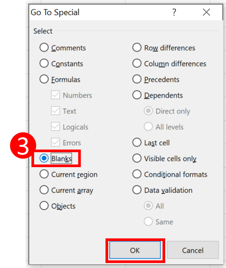
When you finished pressing “OK”, you will notice that the blank cells in column C being highlighted.
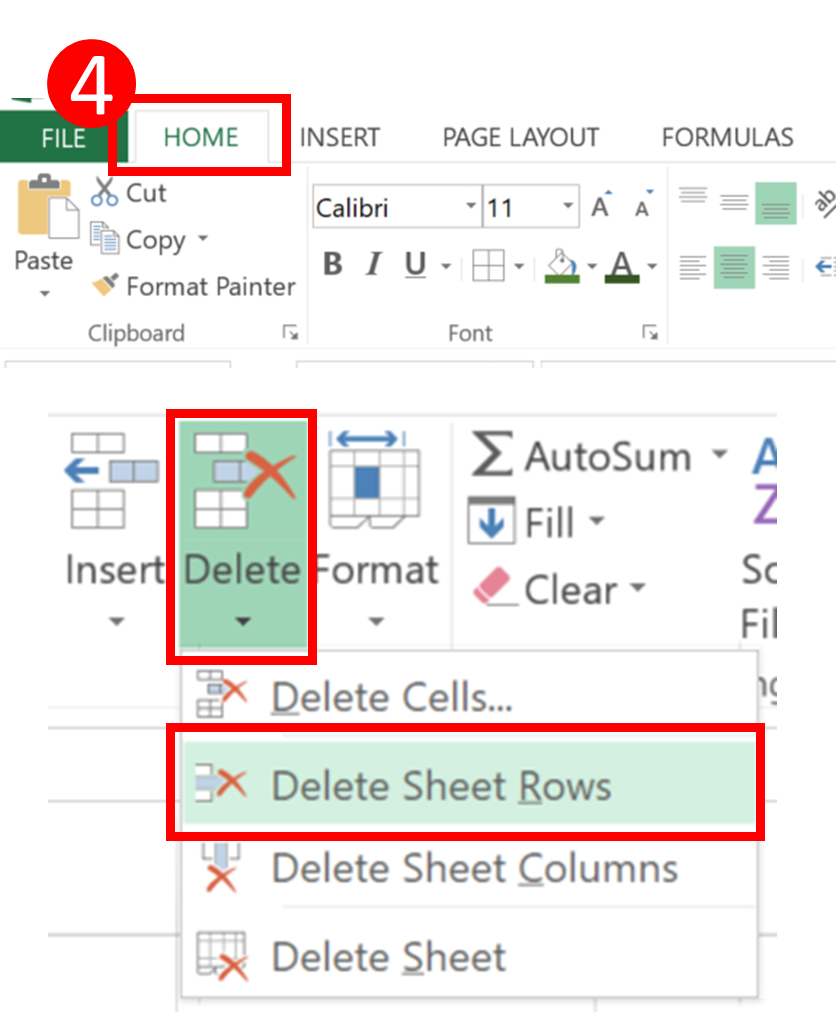
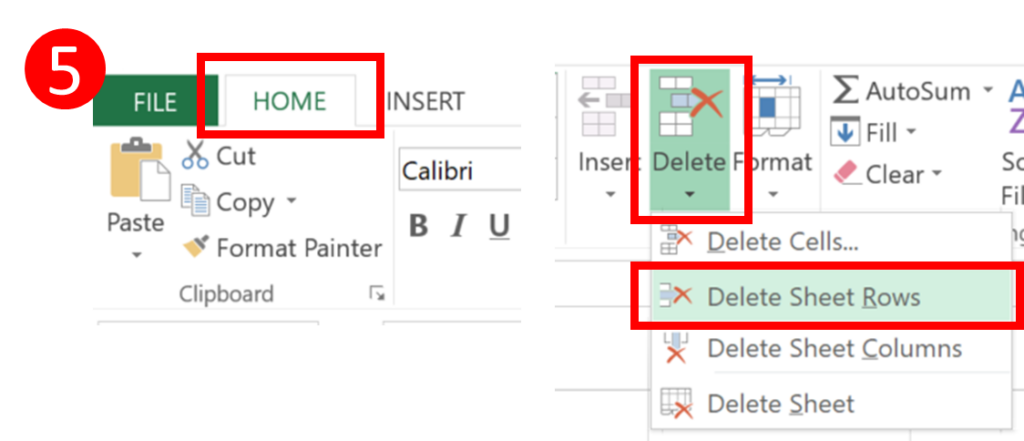
Step 4: Select “Home” > “Delete” > “Delete Sheet Rows”
The shortcut to delete row is Ctrl – (Press Ctrl and minus simultaneously)
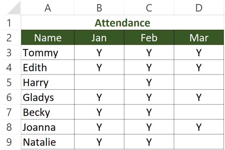
Result
Delete Row if column is Blank by “Sort & Filter”
Step 1: Select the cell range (Including the header)
The first step looks quite similar to the first step in the former solution. Isn’t it?
It may look similar but it is actually not.
Here we need to highlight the header (we don’t need to do so in the former solution).
I will explain it further in step 2.
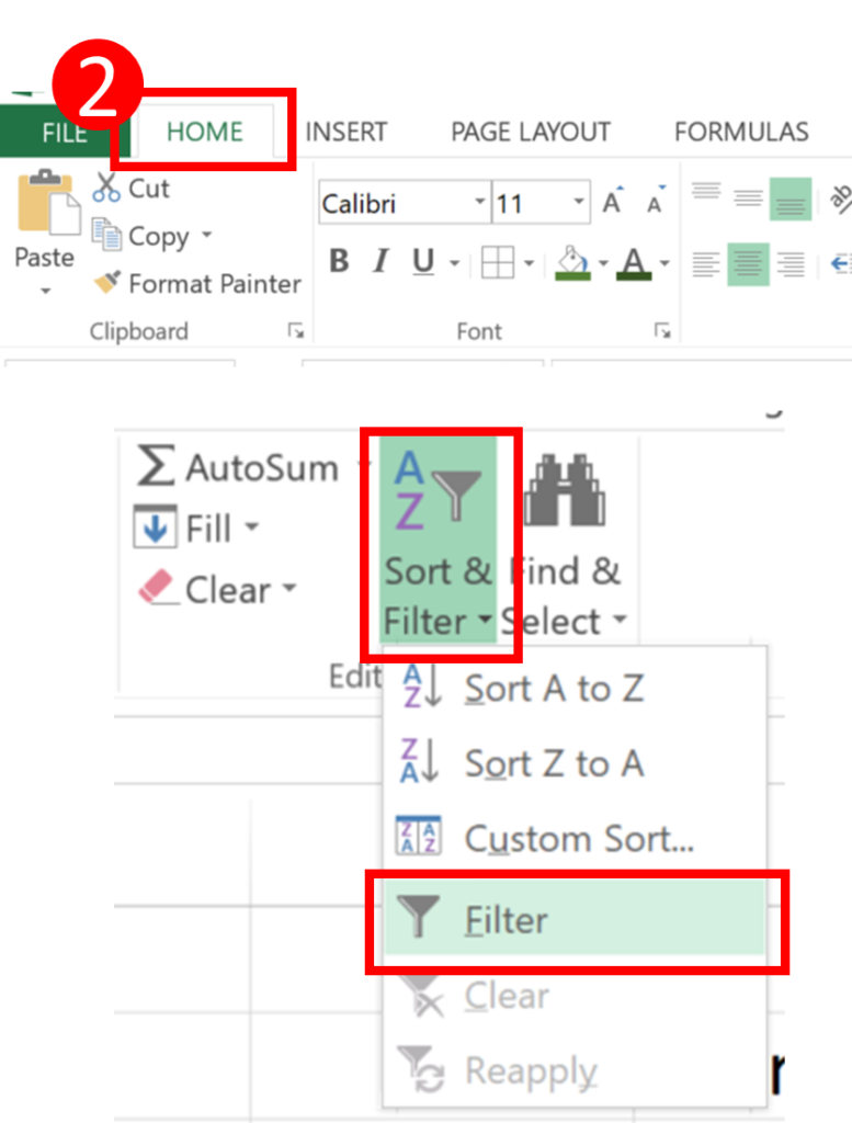
Step 2: Select “Home” > “Sort & Filter” > “Filter”
The shortcut to apply filter is Ctrl + Shift + L. Simply select the column header and apply the shortcut will do.
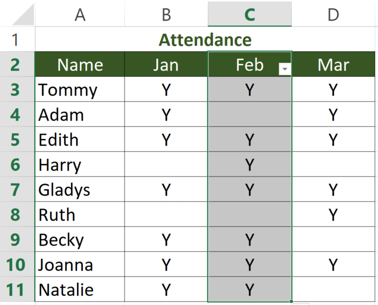
After you apply the filter, the table should look like this.
There is a arrow next to Cell C2, which indicates Cell C2 as a header in the filter table.
You may wonder what it implies. It implies that Cell C2 will be excluded from the all the sorting and filtering when you apply any.
This is why we have to include the column header.
While it may not have a big impact in this case, it could leads to mistakes and miscalculation in other cases.
I suggest you keep this in mind. Including a header in the filter table is usually a good practice.
Before proceeding to next step, you would like to press somewhere else in the worksheet to unselect the current range.
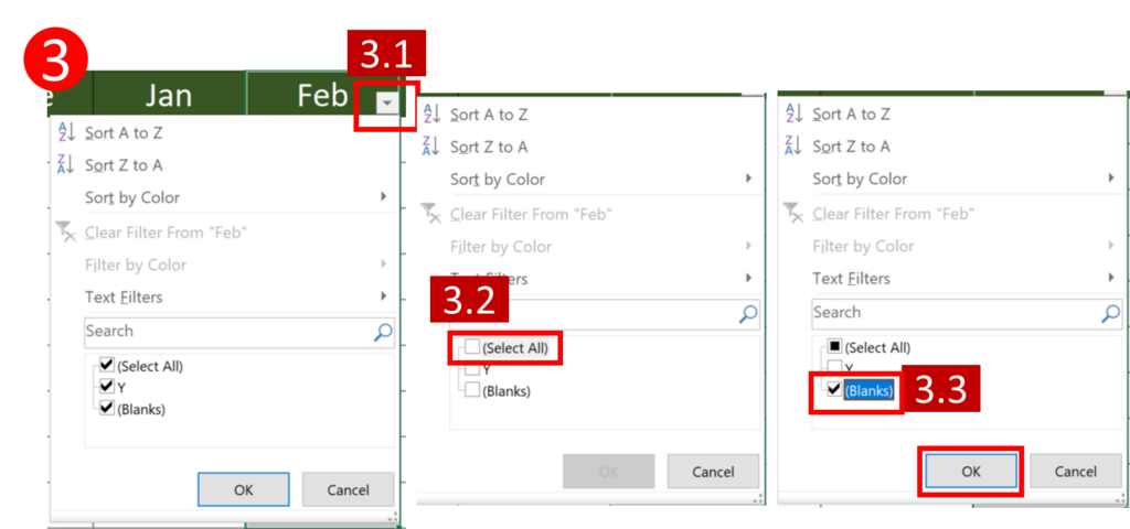
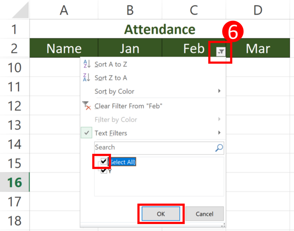
Step 3: Press the down arrow > Uncheck “Select All” > Check “Blanks” > Press “OK”
Here we would like to show rows that contains blank value in column C.
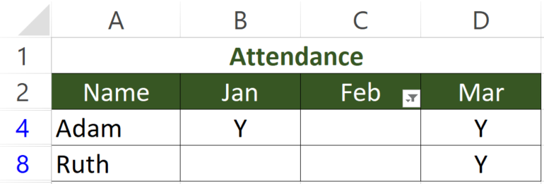
The table should look like this when you finished filtering.
Step 4: Highlight cell range and press Alt ;
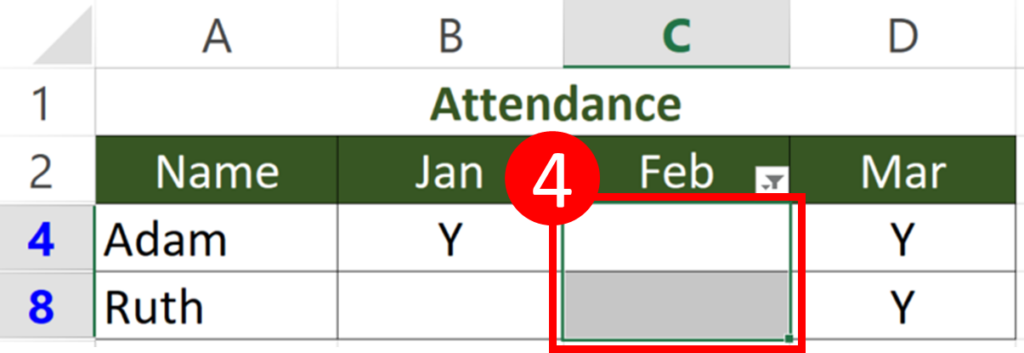
This time we won’t include the column header.
What we want to do is to select the blank cells only.
You may wonder what is this “Alt” key and semi-colon for. This is actually the shortcut to select visible cells only.
When you apply this shortcut, it is not easy to tell that you have successfully apply the shortcut.
Don’t panic if you didn’t see any changes since it is normal.
You can carry out a little test to see if it works – try copy the selection by pressing Ctrl C and then paste it somewhere else. You shouldn’t see anything pasted if the shortcut is working. If something other than blank is pasted, you may want to abandon the shortcut and go for the traditional way instead.
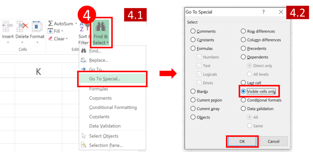
Here is the traditional way:
Home > Find & Select > Go To Special > Visible cells only> OK
Step 5: “Home” > “Delete” > “Delete Sheet Rows”
The shortcut to delete sheet rows is Ctrl – (Press Ctrl key and minus key simultaneously)
Step 6: Press the Filter button > Select “Select All” > Press “OK”
Result
Now we have deleted row which cells in certain column is blank.
You are free to turn off the filter if you wish to.
You might also be interested in 6 Ways To Converting Text To Number Quickly In Excel
Delete Row if column is Blank by “VBA”
**Read How to Insert & Run VBA code in Excel – VBA101 if you forget how to insert VBA code in Excel.
Sub DeleteRowsIfCertainCellIsBlank()
    'Dollar Excel 20220704
    'This VBA code will delete rows if cells in certain cell area is blank

    Range("C3:C11").SpecialCells(xlBlanks).EntireRow.Delete
End Sub
What this VBA code does
This VBA code does the exact same thing as the Customize your VBA code Have you noticed the difference between these 2? When we specify column C, not only blank cells within the table is removed but also the table header. This is because cell C3 is also blank. The table header actually resides in Cell A1. When we specify column C, we will delete everything in column C. I suggest you to be very sure if you want to specify a column instead of a cell range. Although this is what I do not intend to teach you in the article, I guess some of you might be interested in twisting the code a little bit to achieve different results. How to Check/Test if Sheets Exist in Excel? How To List All Worksheets Name In A Workbook How to Unpivot or Reverse Pivot in Excel You might also be interested in How To Remove Digits After Decimal In Excel? Hungry for more useful Excel tips like this? Subscribe to our newsletter to make sure you won’t miss out on any of our posts and get exclusive Excel tips!Specify a column instead of a cell range
Columns("C").SpecialCells(xlBlanks).EntireRow.Delete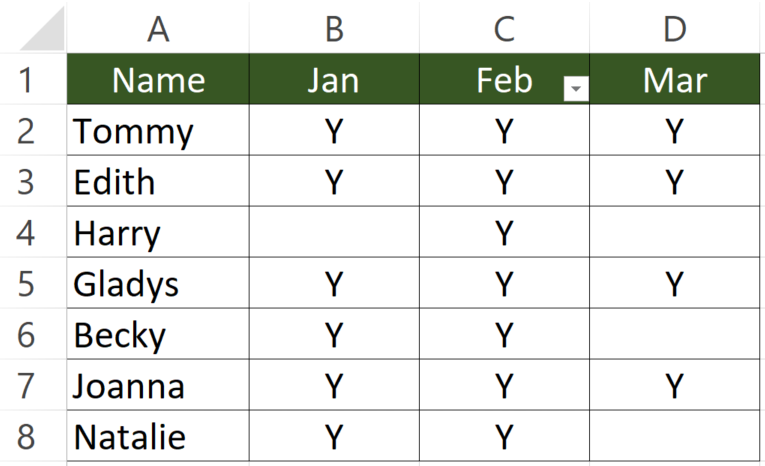
Make the background colour red instead of deleting
Range("C3:C11").SpecialCells(xlBlanks).EntireRow.Interior.Color = RGB(255, 0, 0)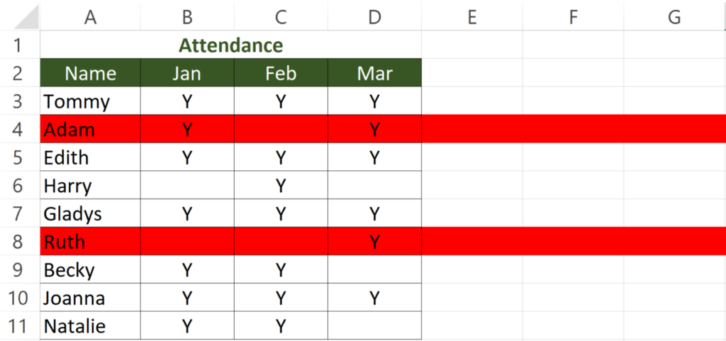
Other VBA articles