We all know that we can highlight cells that equal to specific value by conditional formatting. Is there a way that allows us to highlight cells that equal to more than just one value?
Example

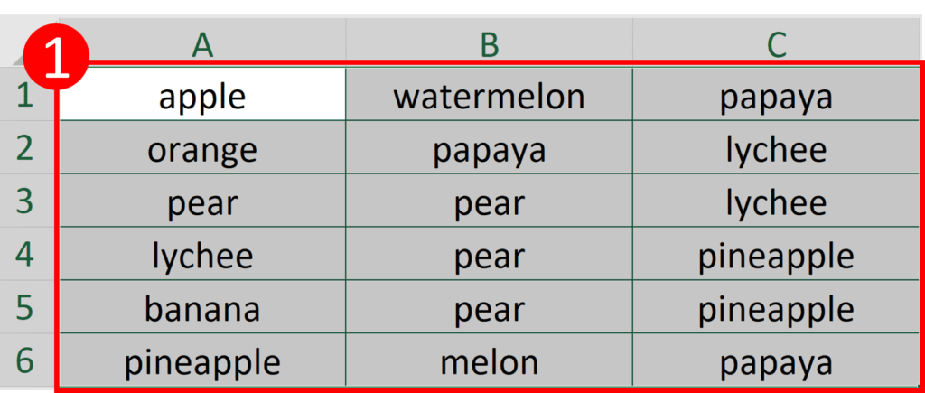
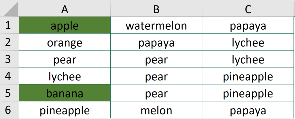
In this article, we will be using this table as an example.
By the end of this article, you will be able to highlight cells that equals to “apple” and “banana” at once.
Why you should learn this method
Basic conditional formatting allows you to highlight cells that equals to one specific value at a time.
Without learning the advanced method, you will need to start the operation again and again. If you happen to need to highlight cells that equals to 20 different values, you will have to do the basic conditional formatting for 20 times.
You may be interested in How To Remove Digits After Decimal In Excel?
How to highlight cells that equal to multiple values in Excel?
To achieve that, you should use conditional formatting. By inputting a formula in conditional formatting, you will be able to identify cells that equals to more than one value at once.
Step by step tutorial
Step 1 Highlight all the cells
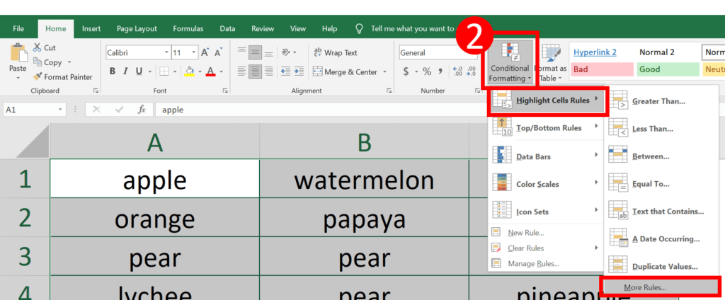
Step 2 Select Conditional Formatting > Highlight Cells Rules > More Rules
You may be interested in How to Show Zeros as Blank Cells In Excel
Step 3 Select “Use a formula to determine which cells to format”
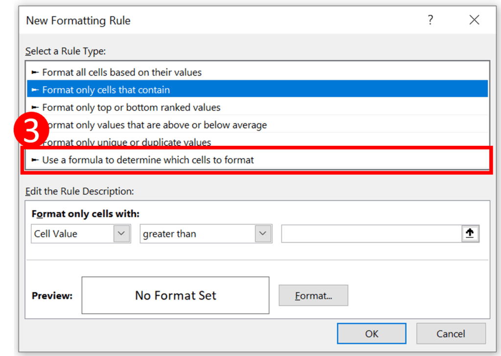
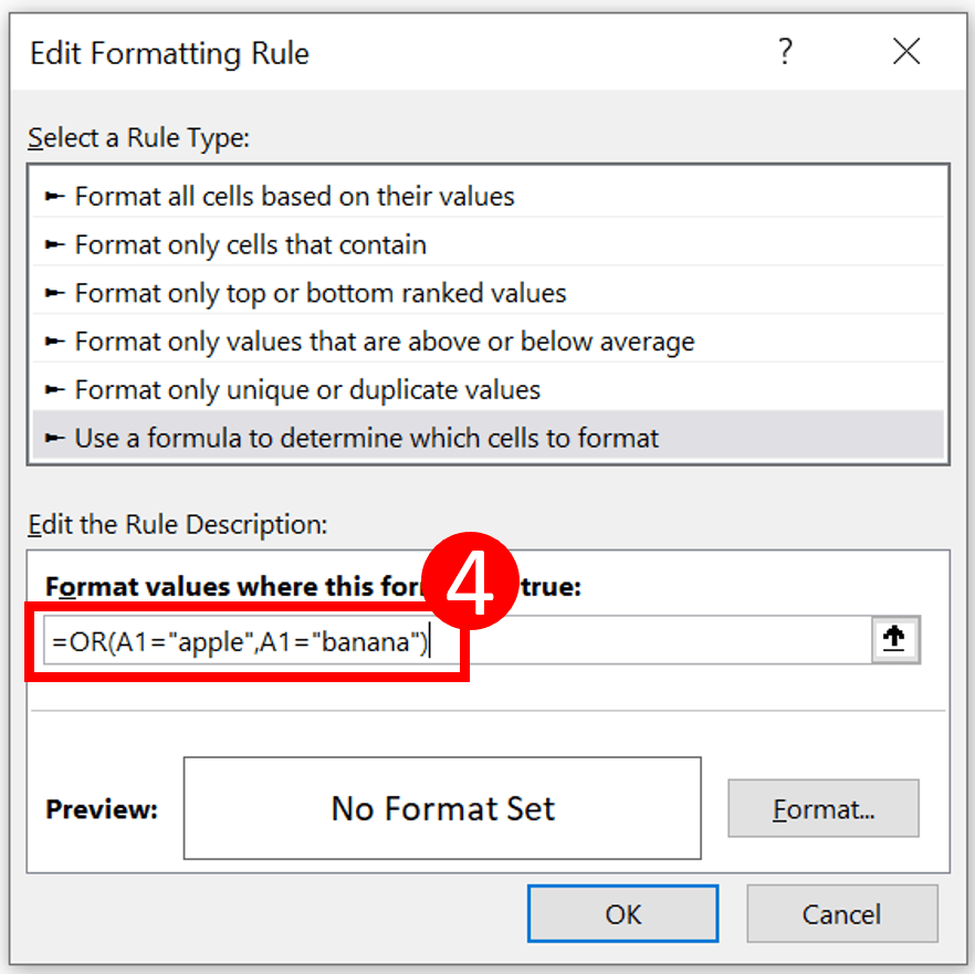
Step 4 Enter the following formula
=OR(A1="apple",A1="banana")
This formula ask Excel to highlight cells equivalent to either “apple” or “banana”.
You can enter as many value as you like.
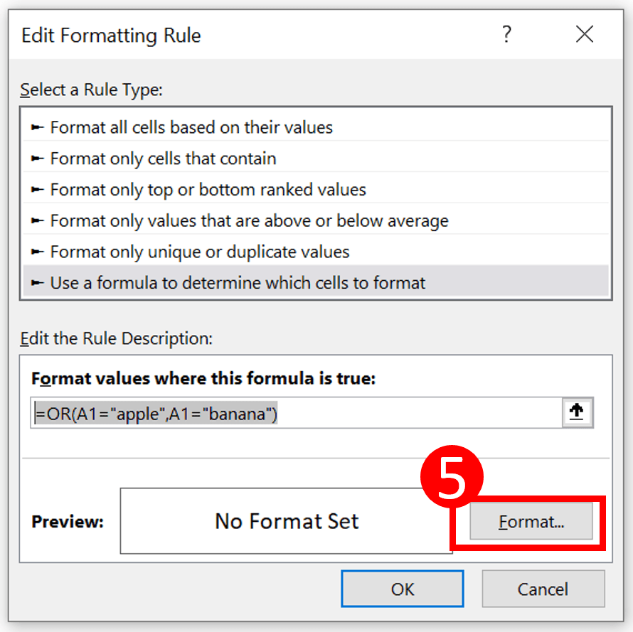
Step 5 Select “Format”
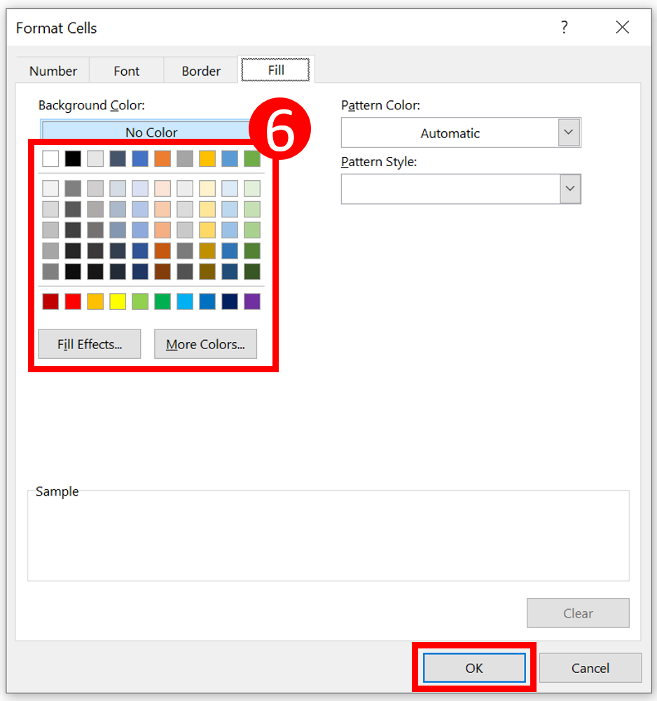
Step 6 Format it as you wish and press OK
This step determines how your cell will turn out if it matches your criteria.
Here I will fill the cell color in green. You can format it however you like it to be.
Press “OK” when you finish formatting.
Result
You may be interested in How to use REPT functions to the Most.
Hungry for more useful Excel tips like this? Subscribe to our newsletter to make sure you won’t miss out on any of our posts and get exclusive Excel tips!