Freeze Panes function allows us to freeze certain rows and columns so that we can view our Excel workbook easily. However, there isn’t any function that allows us to directly freeze top and bottom row at the same time.
In this article, I will show you two workarounds to freeze header row and bottom row. One of the solutions is with table and another one is without using table.
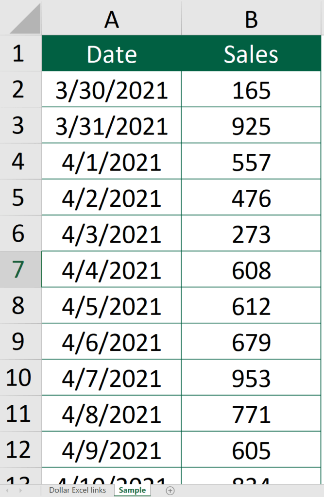
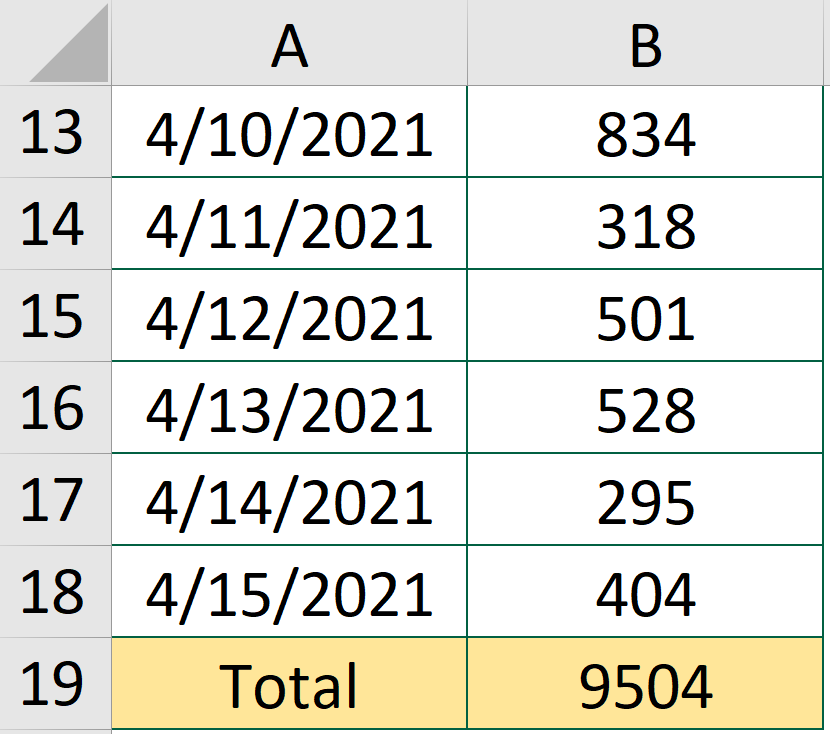
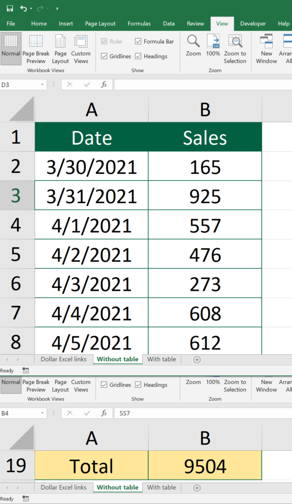
Here is the sample. There are a total of 19 rows of data.
You may be interested in How to highlight cells that equal to multiple values in Excel?
Sample
What we would like to do
To freeze row 1 and row 19 so that we can view them without scrolling up and down.
Freeze top and bottom row without table
Step 1: Select New Window
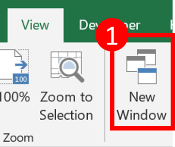
After that, a new Excel window should pop up.

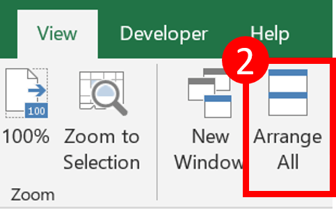
Step 2: Select Arrange All
You may be interested in How to Sum and Count Cells by Color in Excel?
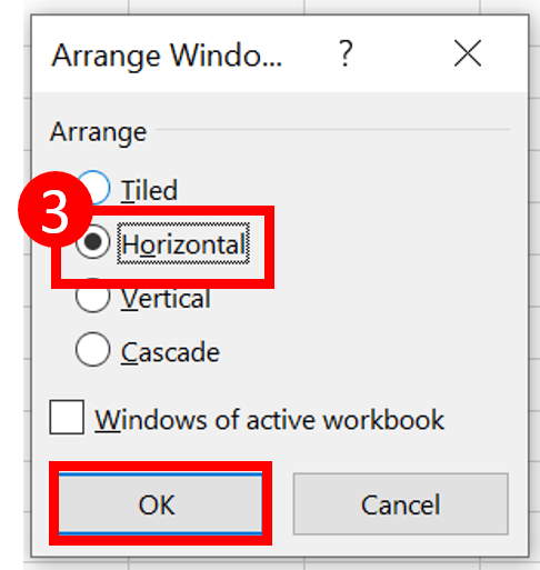
Step 3: Select Horizontal and press OK
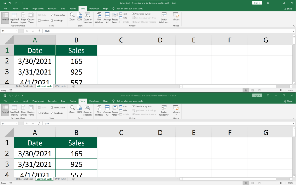
Now your Excel should look like this. There are two Excel windows showing exactly the same Excel document. You can adjust the height of each window by dragging the edge of the window.
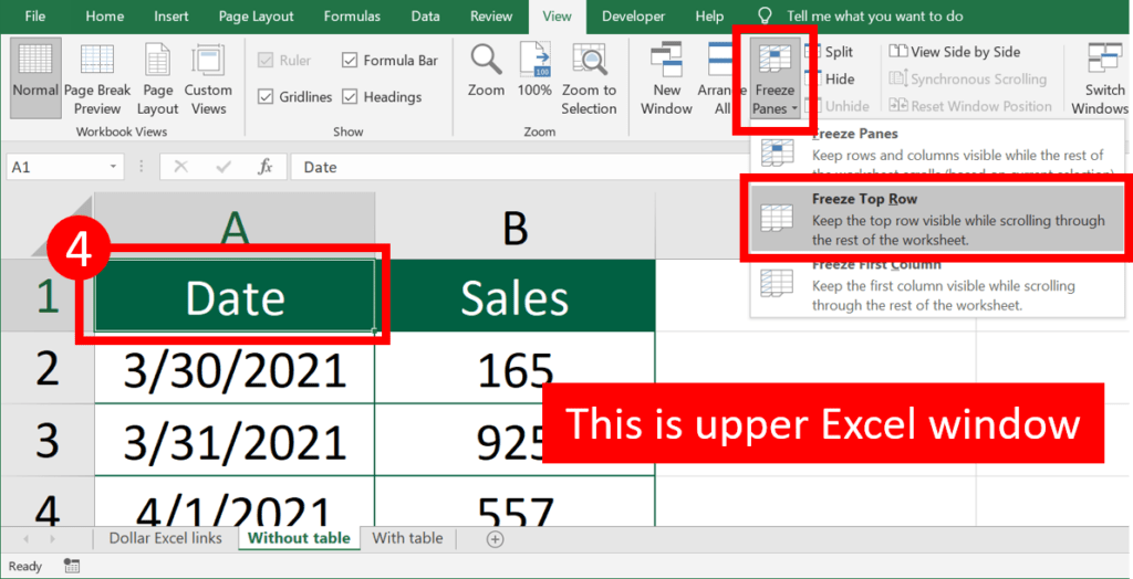
Step 4: Select cell A1 and select Freeze Panes > Freeze Top Row
Here we are talking about the upper window.
This step will freeze the top row of the upper window.
Step 5: Select Lower Excel window and scroll down to the last row
And you are done!
You may be interested in How to Sum and Count Cells by Color in Excel?
Freeze top and bottom row with table
Step 1: Select the data range
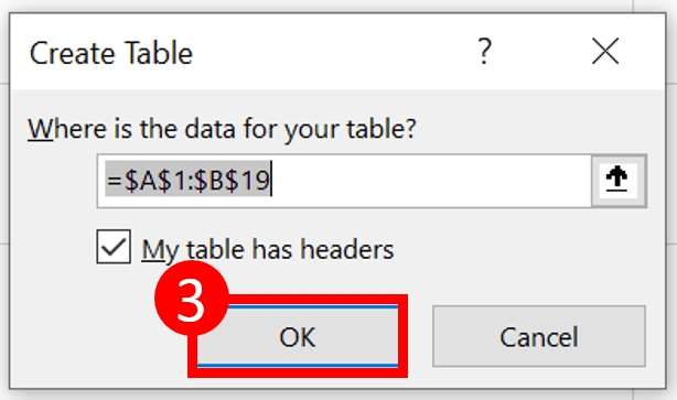
In the sample, the data range is A1 to B19.
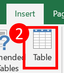
Step 2: Select Table
Step 3: Press OK
Now your data range has turned into a Excel table. When you scroll down, you will realise that the column header is taken over by cells at row 1. Instead of “A”, the column header now became “Date”.
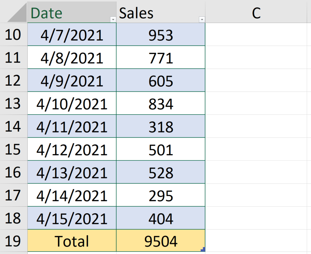
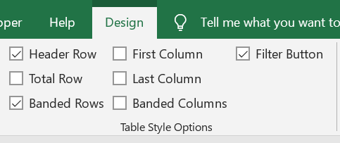
You may notice that the table style and cell colour has changed. You may play around with Table Style Options if you do not like the current table style.
You may be interested in How to Show Zeros as Blank Cells In Excel
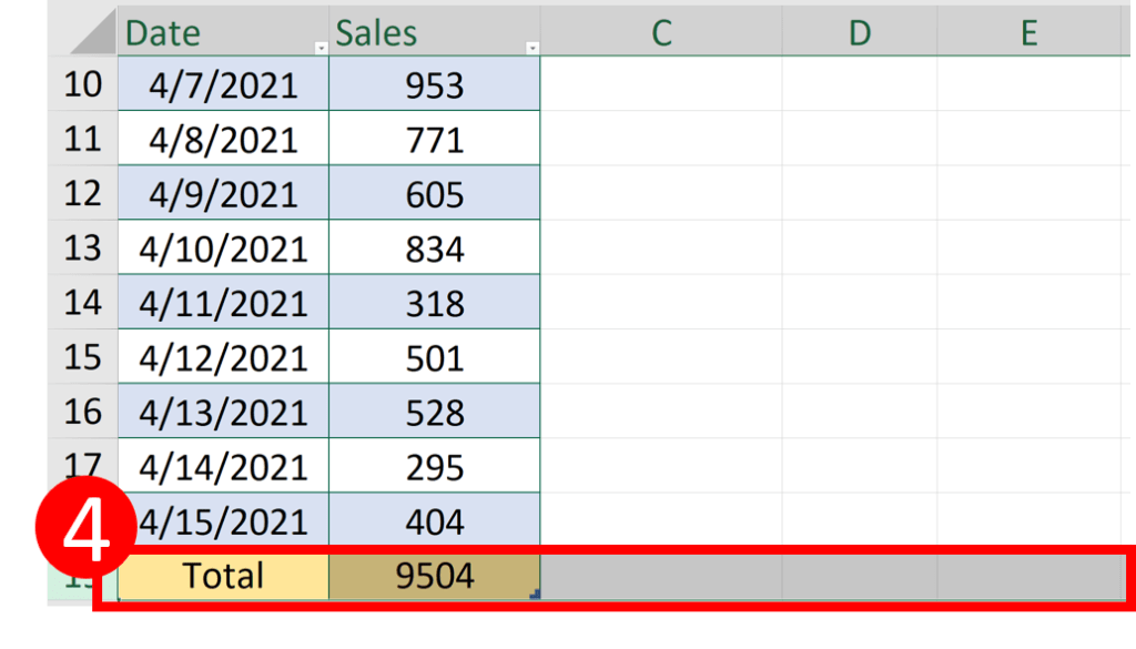
Step 4: Select the entire bottom row
There are two ways to select the entire row.
- Press the row number
- Press any cell on the row and press “Shift space space” (Do not release the “shift” key until you finished pressing “space” twice)
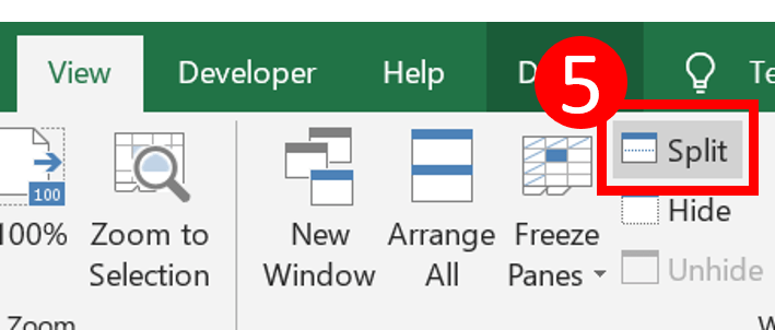
Step 5: Press Split
You may be interested in How to Sum Intersections of Multiple Ranges (Excel)
Step 6: Press Cell A1
You can start to scroll up and down now.
You will realise you can see both top row and bottom row now.
Hungry for more useful Excel tips like this? Subscribe to our newsletter to make sure you won’t miss out on any of our posts and get exclusive Excel tips!