Only a few Excel users know about that we can create graphs with REPT function.
Most people use the REPT function simply to repeat characters but the REPT function actually does much more than that.
Some people think the REPT function is similar to the sparklines feature since they both create an in-cell chart and argue that sparklines win over the REPT function. I don’t try to rank one over another. It depends.
Compare to a normal chart, an in-cell chart makes things easier in terms of alignment. You don’t need to worry that inserting rows or deleting rows may mess up the spreadsheet.
In this article, I will show you how 5 types of graphs to create with the REPT function. They are star rating chart, dot chart, bar chart, tally chart, and mirror graph.
Sample workbook
Star rating
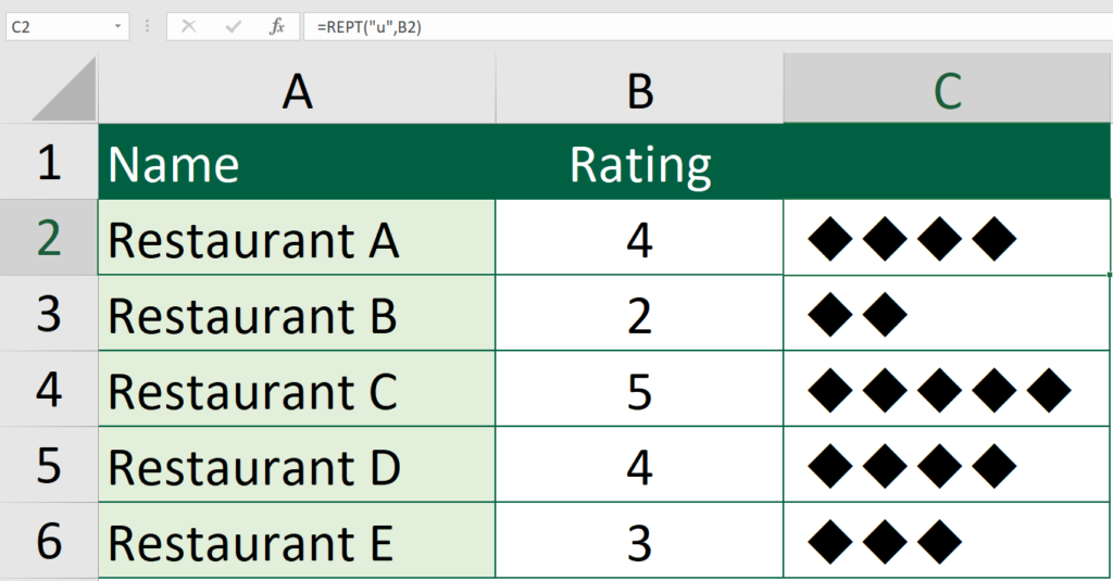
Formula of cell C2
=REPT("u",B2)Ever wonder that you can make a simple star rating system with Excel?
The usage of REPT function is nothing special here. The choice of font is what makes it special.
The font of cell C2 through cell C6 is “Wingdings“. This font enables you to insert special symbols. In the above example, I typed “u” in the cell and spade is shown.
The following table has gathered some frequently used symbols. For example, if you would like to insert a smiley face, you should type a “J”.
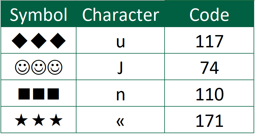
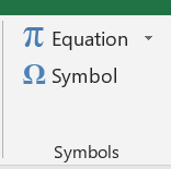
If you would like to choose among different symbols, go to “Insert” tab, press “Symbol”. Then a symbol window should pop up.
You might also be interested in Edit The Same Cell In Multiple Excel Sheets
Dot Chart
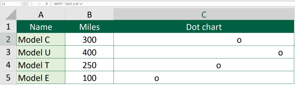
Formula of cell C2
=REPT(" ",B2/5-1) & "o"For this chart, you don’t need to change the font. You could replace the “o” with other characters.
Bar Chart

Formula of cell C2
=REPT("|",B2)This is another “font tricks”. I simply set the font as “Playbill” and I get the amazing result.
You might also be interested in How To Convert Cells Range To Image In Excel
Tally Chart
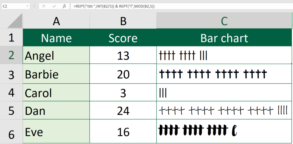
Formula of cell C2
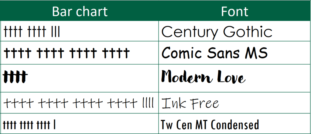
=REPT("tttt ",INT(B2/5)) & REPT("l",MOD(B2,5))Using REPT function along with INT function produce a tally chart. To make a tally chart with a different style, you can play around with the choice of font. Here I suggest five fonts to be used. “Tw Cen MT Condensed” makes the tally chart looks a bit formal while tally chart with “Modern Love” looks a bit playful.
Mirror Graph
Formula of cell D3
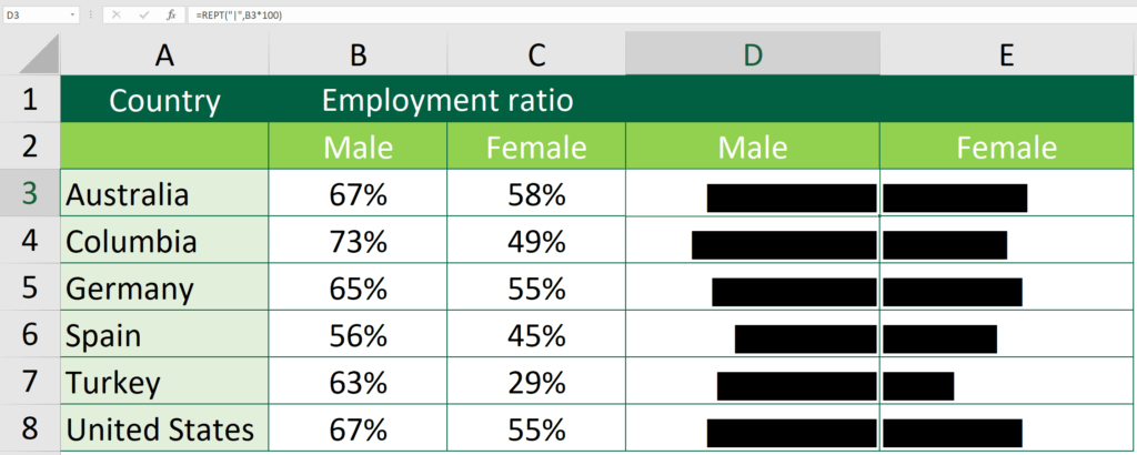
=REPT("|",B3*100)Formula of cell E3
=REPT("|",B3*100)The catch here is the alignment of cells. Making a mirror graph is as easy as aligning the left bar chart to the right and aligning the right bar chart to the left. The reason I love Excel so much is that different results can be produced with a little tweak.
Hungry for more useful Excel tips like this? Subscribe to our newsletter to make sure you won’t miss out on any of our posts and get exclusive Excel tips!