Background
Zeros are almost inevitable in a workbook.
Sometimes you may change the appearance of the zero.
Do you have the following ask?
- Display zero as blank cells
- Show zero as dash
- Hide zero without actually deleting zero
In this article, I will show you 4 ways to hide zero cells or replace them with blanks or other marks such as dash.
Pros & Cons (4 ways)
| Method | Advantage | Disadvantage |
|---|---|---|
| Change Excel Setting | Changes are applied to the whole workbook | You couldn’t change for a single worksheet |
| Find & Replace | It replaces 0 by blanks | / |
| Use a formula | It is dynamic | It only works if the cell contains a formula |
| Change number format | It hides 0 instead of replacing it by blanks | It doesn’t replace 0 |
Example
Sample Workbook
Download the workbook to practice it by yourself!
The sample workbook have included the practice worksheet for each option.
You can press the button and download it. (Only available in Desktop version)

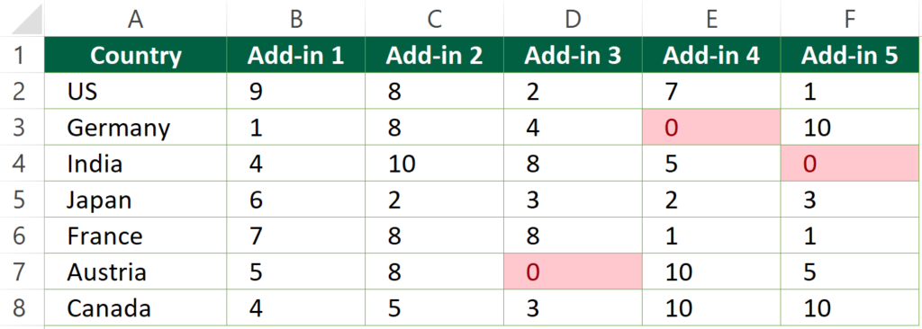
Expected Outcome

Option 1: Change Excel Setting
This will change the setting for the whole workbook.
If you just want to show zero as blank cells for a specific cell range, skip this option.
Step 1: Choose File tab
Step 2: Choose Options
Step 3-5: Choose Options
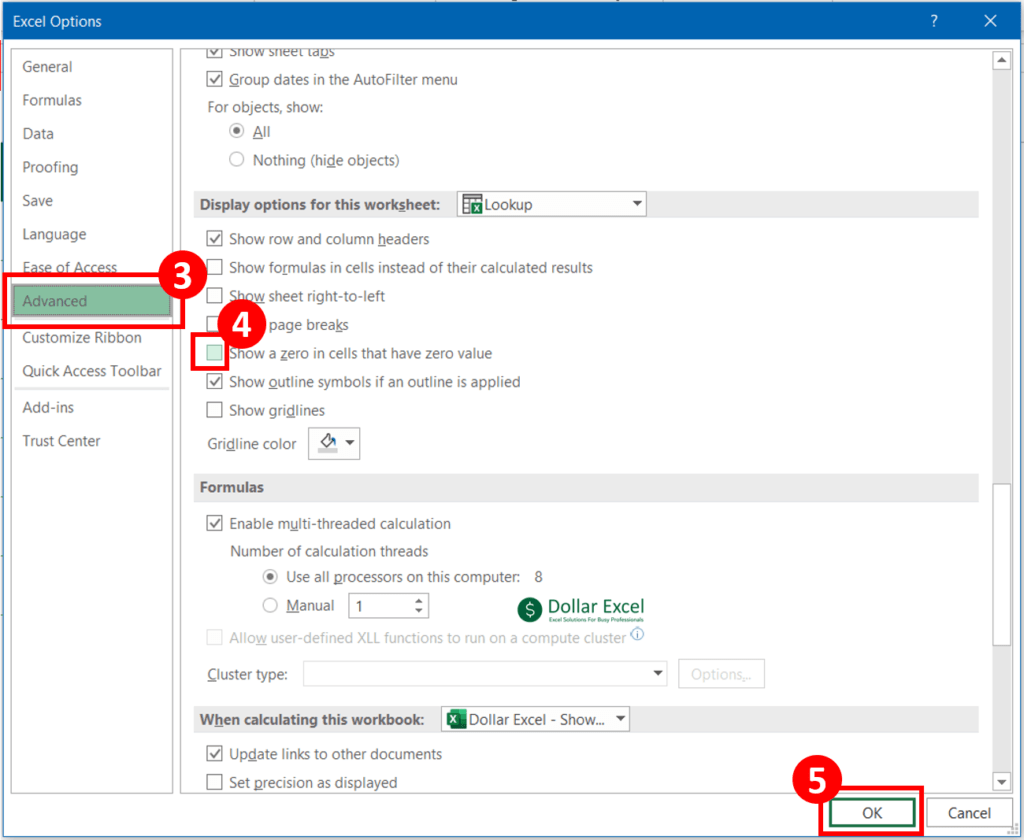
Step 6: Done
Option 2: Find and Replace
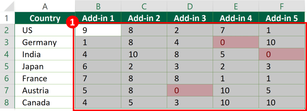
Step 1: Select cell ranges
Step 2-3: Type the 0 into Find what box and press Replace all
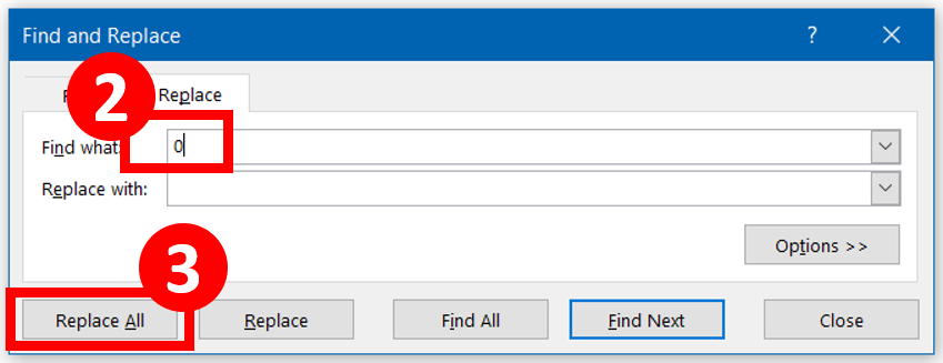
Step 4: Close the “Find and Replace” dialog
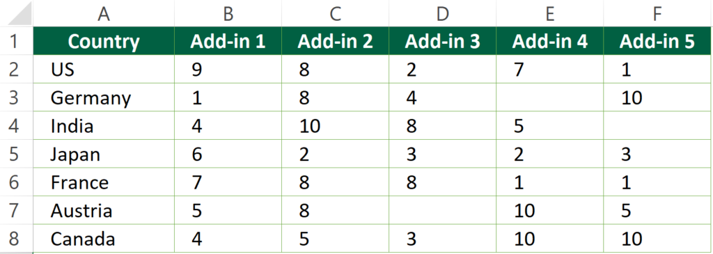
Step 5: Done
Result of option 2
Option 3: Use a formula
If the cell ranges contains formula, you can use a formula to wrap around the original formula.
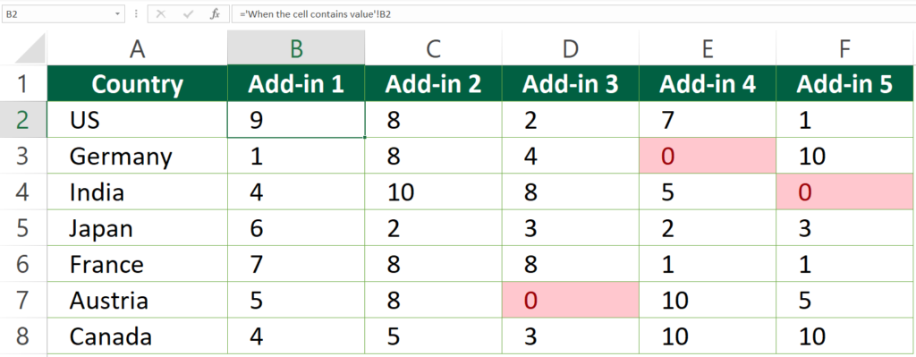
Step 1: Identify the formula
As you can see, the original formula is
='When the cell contains value'!B2
Step 2: Revise the formula
=IF('When the cell contains value'!B2=0,"",'When the cell contains value'!B2)The logical of the formula
- To identify if the value is 0
- If the value is 0, then make it blank
- If it is not 0, resume the original formula
Step 3: Drag the formula to remaining cells
Result of option 3
Option 4: Change number format
Step 1: Select cell ranges
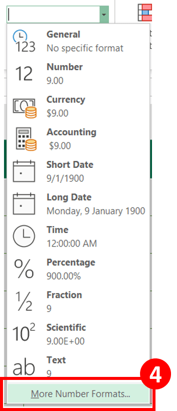
Step 2-3: In home tab, select the number formatting triangle
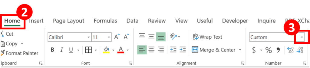
Step 4: Select More Number Formats
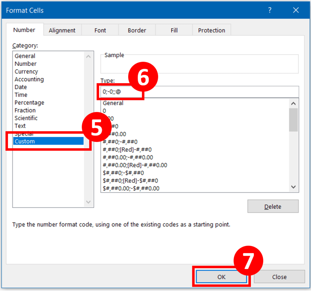
Step 5-7: Select “Custom”, type this into format box and press “OK”
0;-0;;@
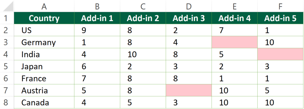
Result of option 4
Hungry for more useful Excel tips like this? Subscribe to our newsletter to make sure you won’t miss out on any of our posts and get exclusive Excel tips!