Background
If you follow through our introduction to the binomial option pricing model (Part 1 and Part 2), you’ll notice that the binomial model is a discrete-time model, meaning that the uncertainty of the stock price movement is bound in discrete period like year 1, 2, 3 and month Jan, Feb, Mar etc. A natural question to ask is if we can work on continuous periods instead of discrete, something more like our daily experience?
This article would be more conceptual at first, but we’ll tie this with a calculated example applying the Black-Scholes equation.
Sample Workbook
As always, feel free to download our sample workbook to work through the examples with us.
You may also be interested in How to Display the Formula as Text in Excel?
Brownian Motion
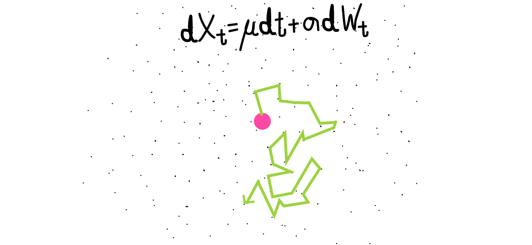
Financial modelers aim to answer this with what we call a continuous-time stochastic model, which is a fancy word to frame our question above. Borrowing from Physics, financial modelers based their modelling of the stock price with what we call a Brownian motion/diffusion – a random process that is closely related to the Normal Distribution. Brownian motion is first used to describe how a pollen grains move randomly after colliding with water molecule, as describe in the figure below:
Black-Scholes Equation & Delta-Hedging
We are going to simplify a lot (really a lot!) of the details in coming up with the B-S equation, but the key idea is to remember what we try to achieve in the binomial option pricing model and generalize the idea into continuous-time. Financial modelers start with the same setup as the binomial tree model: a hedging portfolio. This time, we are instead interested in a dynamic setting, so the delta-hedge (d* in our previous article) is instantaneous and continuous. With some heavy-lifting in stochastic calculus, we arrive at a portfolio that is risk-free, and is able to arrive at the present value through discounting the payoff of the replicating portfolio with the risk-free interest rate.
One of the terms that you’ll often hear people mention is the lognormal distribution. Because of the close relationship of the Brownian motion and the Normal distribution, we are de facto modelling the stock returns (or more precisely, the log-returns) using the normal distribution. As such, the stock price at a after a given period of time will follow a lognormal distribution, which is a skewed and non-zero.
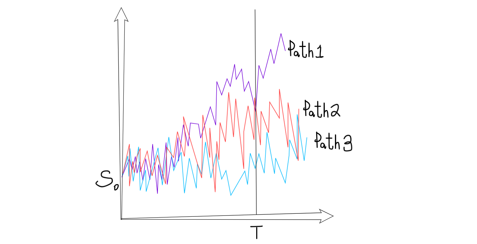
An important thing to note here is on the form of the solution of the option price. While a nice pricing equation does exists for in more vanilla options which are not path-dependent (i.e. you could not exercise the option mid-way through the contract), they don’t exist for exotic products which are path-dependent. In those cases, we’ll have to use a technique called Monte-Carlo Simulation to approximate the price.
You may also be interested in How to Sum and Count Cells by Color in Excel?
Under Black-Scholes, stock price is assumed to be distributed lognormally.
European Options – With nice equations
Since European options are not path-dependent, we do have nice equations to describe their price under the Black-Scholes model. This is again a result of modelling the stock price under a lognormal distribution (which comes from the Brownian Motion), and therefore we can deduce a general pricing formula for European options. If you are interested in the derivation, you can check it out at the end of this article, but otherwise we’ll take the results as granted and apply it to Excel.
Let’s start from the pricing input:
- S0: Initial stock price
- K: Strike price
- r: Risk-free rate of interest
- σ: Volatility of the stock
- T: Time to maturity
Given the following input, the appropriate (i.e. no-arbitrage) price for a European call option is provided by applying the formula shown below. Don’t be discouraged by the seemingly complicated formula! As usual, let’s give the components a economic interpretation and understanding the concepts behind.

At first glance, you may notice that the formula is in the format similar to the payoff of a call option, which is S – K. The only difference is the N(d1) or the N(d2) that is applied to S and K separately. While the math is complicated, the intuition is:
- S0N(d1) is the conditional expected value of the stock price at maturity, given that the option is in-the-money
- N(d2) is the probability of in-the-moneyness, i.e. the expected value of the price you paid for the stock at maturity is the discounted strike price multiplied by N(d2)
You may also be interested in How To Reverse Concatenate In Excel (3 ways)
European Option in Excel
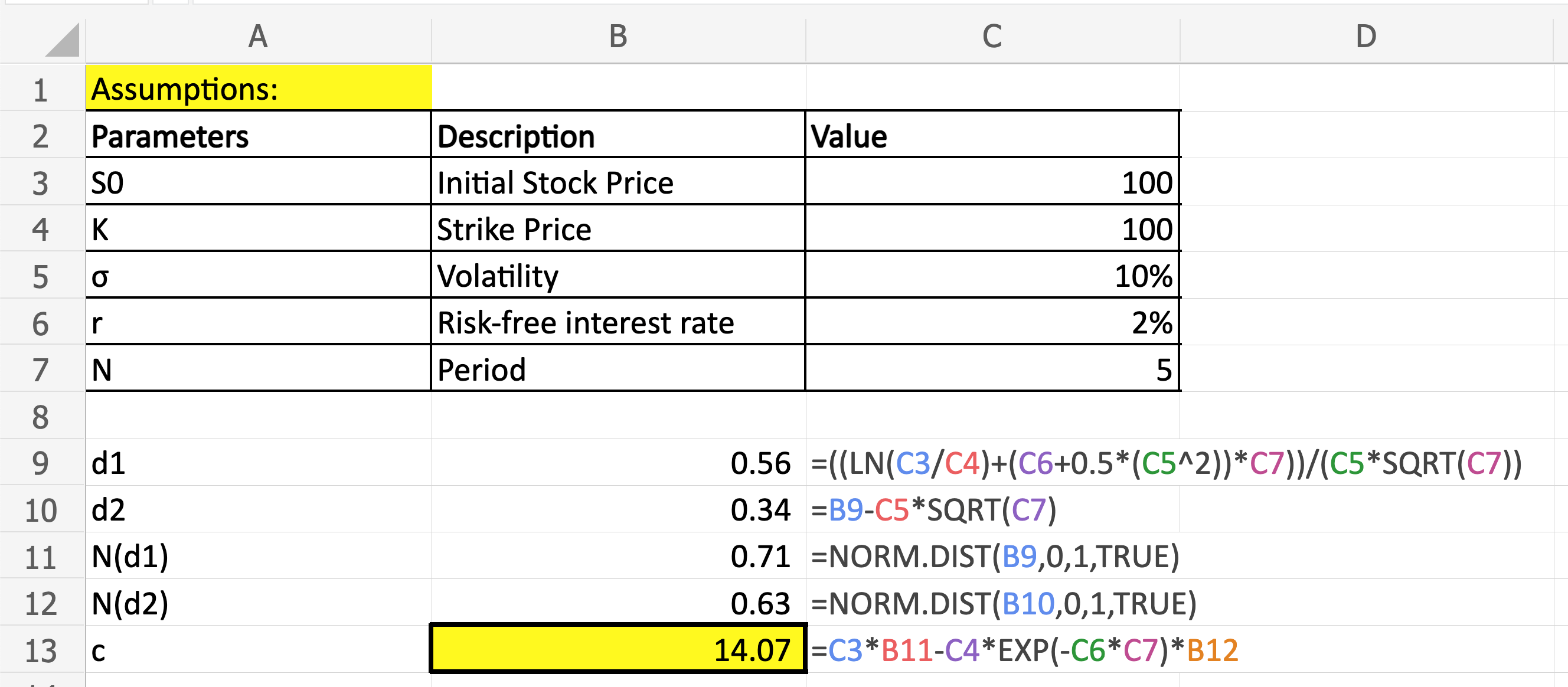
Applying the formula we have in the above, we can easily price any European option as long as we have the 5 inputs available to us! One thing to keep in mind here is on N(d1) and N(d2). Since we are trying compute the cumulative probability function of a standard normal random variable at d1 (or d2), we need to use the Excel functions =NORM.DIST(d1,0,1,TRUE), where 0 and 1 are the mean/standard deviation of the Normal distribution respectively.
Try it out yourself and see if you can get the formula correct in Excel!
What’s Next?
In our next article, we are going to introduce an even more sophisticated and interesting way to price options in Excel – Monte-Carlo Simulation. We’ll start with an example for American option and work our way to learn about VBA as well.
You may also be interested in 2021 New Year Resolution List for Excel
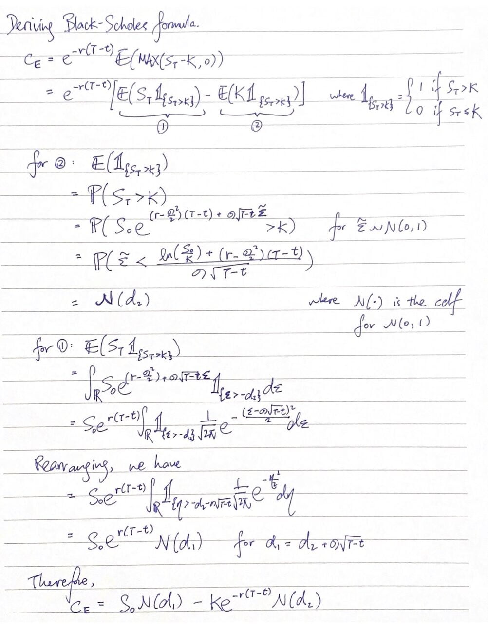
Appendix: Deriving the Black-Scholes formula
This part is for the geeks: we outline a proof to arrive at the Black-Scholes formula for pricing an European call option below.
Hungry for more useful Excel tips like this? Subscribe to our newsletter to make sure you won’t miss out on any of our posts and get exclusive Excel tips!


