


Background
Sometimes we may want to sum and count cells based on background colour of a cells.
I personally don’t suggest using background colour frequently. I do think background colour has its advantage. You can check out 5 Golden Rules for Excel Formatting to see how to format Excel better.
It is such a pity that we don’t have a function or formula for distinguishing between different colours.
The most popular way of summing coloured cells is to use VBA to create a user-defined function to identify the colour code of a cell. However, not every Excel users are familiar with VBA and not all of them prefer using a VBA because of different concerns.
In this article, I will show you how to sum and count cells by colour without VBA.
You might also be interested in Edit The Same Cell In Multiple Excel Sheets
Example
Sample Workbook
Download the workbook to practice it by yourself!

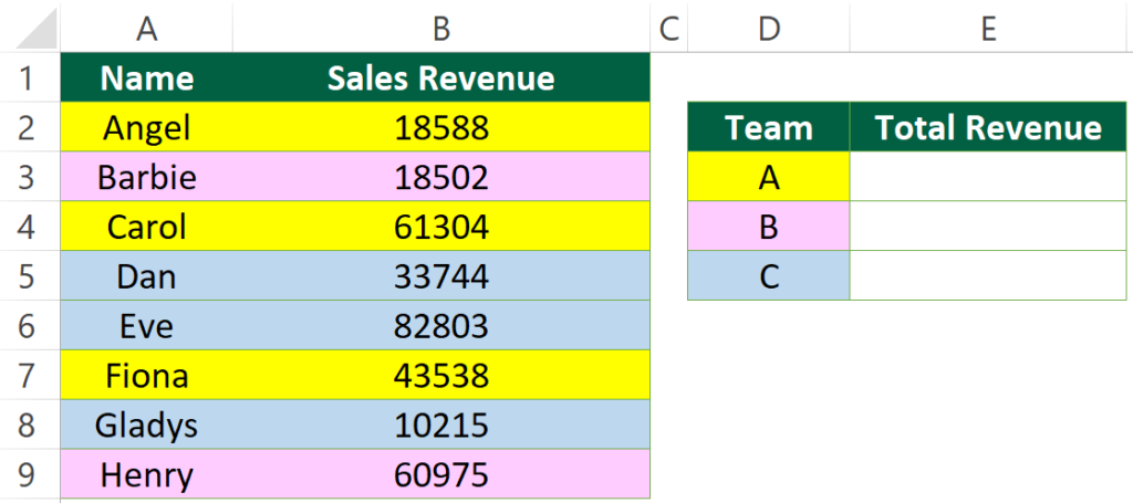
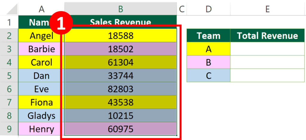
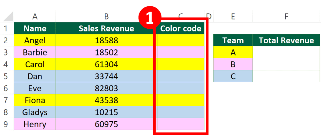
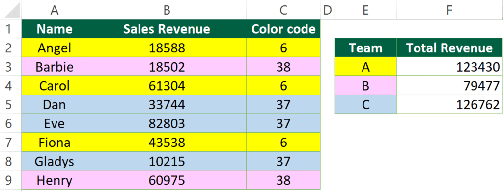
In the example, the background colour of a cell has indicated the team each sale belongs to. For example, Angel belongs to Team A, Barbie belongs to Team B.
What we want to find out is the total revenue for each team.
Of course we can calculate it manually simply by using SUM function and selecting each cell one by one. But that only works if we have a small data set. If we have hundreds of rows, it may result in errors and waste of time.
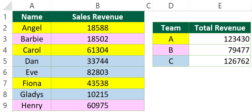
Expected Outcome
The expected outcome is like this. We get the total revenue for each team.
Option 1: Define Name and SUM()
You may also be interested in Look Up the Last Value in Column/Row in Excel
Step 1: Select cells range
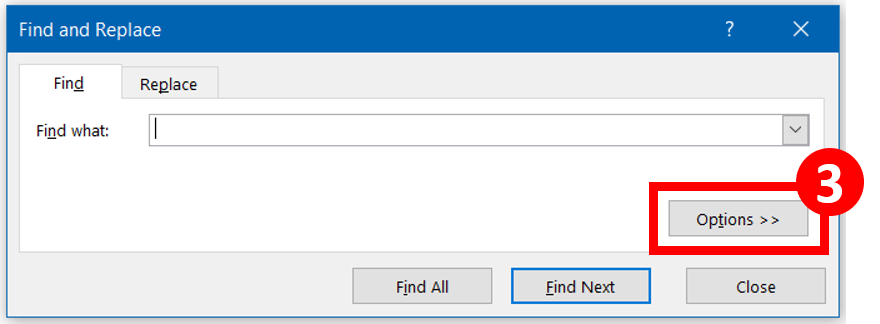
Step 2: Press Ctrl + H to open the “Find and Replace” dialog
Step 3: Press “Options >>”
This step enables advanced Find & Replace options.
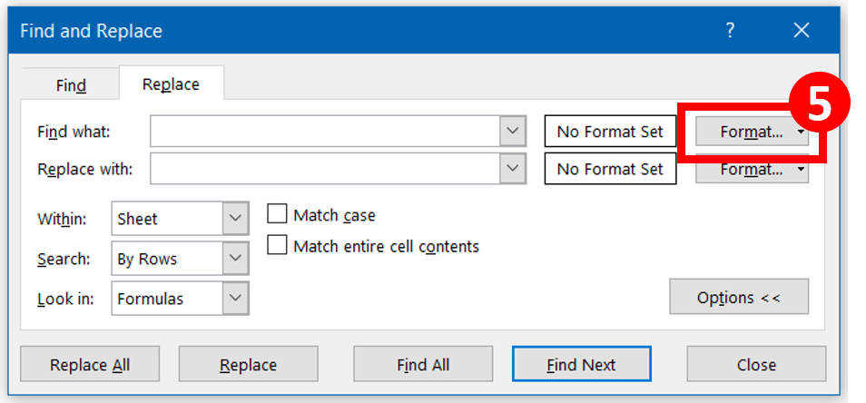
Step 5: Press “Format…”
Most of the Excel users do find and replace by inputting text. In fact, Excel allows you to do matching by choosing a specific format.
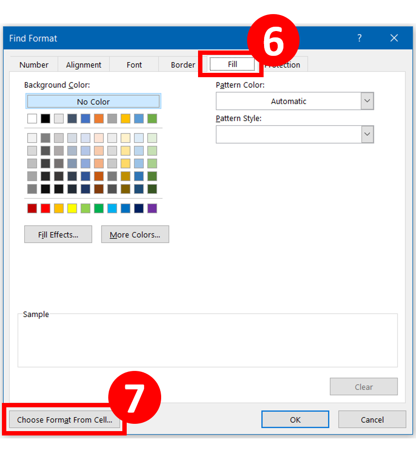
Step 6-7: Choose “Fill” tab and press “Choose Format From Cells”
Choosing different formats one by one can be time-consuming. Instead, there is a cool feature called “Choose Format From Cell…”.
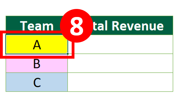
Step 8: Choose the coloured Cell
By pressing the button, you don’t need to choose the background colour or font colour. All you need to do is to choose a cell that has the same format as what you are searching for. Isn’t it cool?
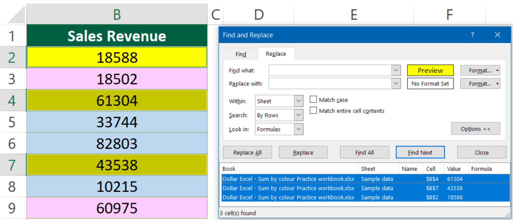
Step 9: Press Ctrl A to select all matching results
Ctrl A is the shortcut for “Select All”. Now you have identified the cell with yellow background by advanced Find and Replace. Ctrl A will enable you select all matching results.
Step 10: Type a name into Name box
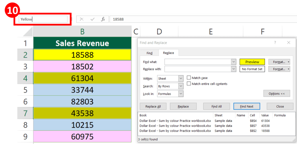
For remaining colour, you can repeat the above steps.
You may also be interested in 2021 New Year Resolution List for Excel
Step 11: Input the below formula
Formula for yellow team
=SUM(Yellow)
Formula for pink team
=SUM(Pink)
Formula for blue team
=SUM(Blue)
Result
How to count cells by colour?
You simply need to change the formula into COUNT().
Formula for yellow team
=COUNT(Yellow)
Formula for pink team
=COUNT(Pink)
Formula for blue team
=COUNT(Blue)
You may also be interested in How to Generate Random Dates in Excel
Option 2: By Get.cell and Sumif()
Step 1: Insert an auxiliary column
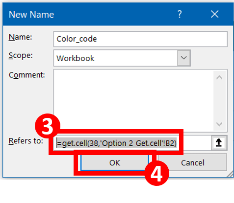
Step 2: Press Ctrl + F3 to open the “New Name” dialog
Step 3-4: Input this formula into Refers to box and press “Enter”
GET.CELL is an early Excel macro function. In recent version of Excel, you could not use GET.CELL directly but there is a workaround. You can use it by defining names.
There are a total of 66 piece of cell information you can get using GET.CELL function.
I will be publishing the article that is solely about GET.CELL soon. Stay tuned.
The serial number of getting background colour code is 38 so we will be inputting that number as the first parameter. The second parameter is the cell we are referring to.
=GET.CELL(38,'Option 2 Get.cell'!B3)
Step 5: Enter this formula
=Color_code
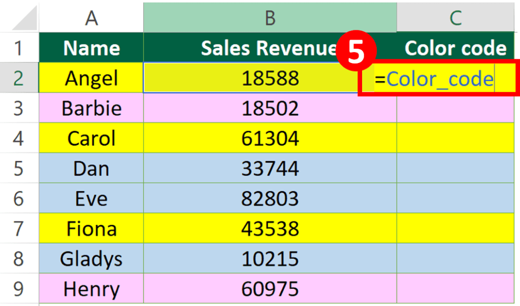
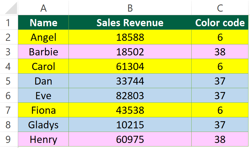
Step 6: Copy the formula down
Now we have the background colour code of each cell in column C.
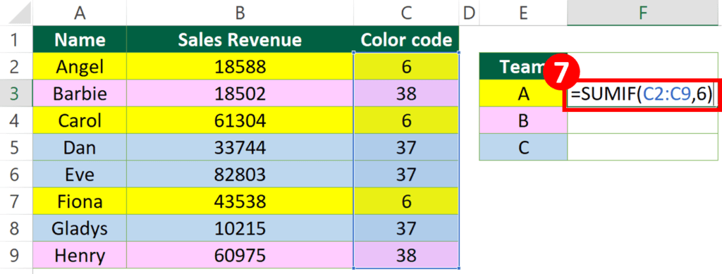
Step 7: Perform SUMIF/ COUNTIF calculations
To sum cells by colour
We can perform SUMIF function with the colour code.
Since the colour code of yellow is 6, we will be inputting 6 into the criteria range of the formula.
Formula for yellow team
=SUMIF(C2:C9,6,B2:B9)Formula for pink team
=SUMIF(C2:C9,38,B2:B9)Formula for blue team
=SUMIF(C2:C9,37,B2:B9)You may also be interested in 6 Ways To Converting Text To Number Quickly In Excel
To count cells by colour
Formula for yellow team
=COUNTIF(C2:C9,6)
Formula for pink team
=COUNTIF(C2:C9,38)
Formula for blue team
=COUNTIF(C2:C9,37)
Result
Things to be aware of:
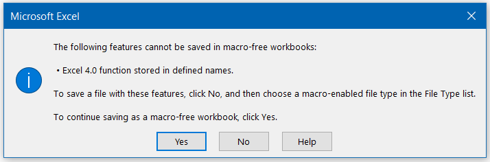
If you went for option 2, make sure you save the Excel workbook in XLSM format or else you will get this warning. This is because GET.CELL function is recognised by Excel as a macro function.
If you prefer to store the Excel workbook as XLSX format, maybe you should try option 1.
Do you find this article helpful? Subscribe to our newsletter to get exclusive Excel tips!