You may have a workbook that have cells filled with different colour.
It is easier to deal with if the colour is a part of the conditional formatting.
If it is not, things got a lot more complicated.
Do you have the following questions?
- How to select cells that are filled with colour?
- How to filter cells that are filled with colour?
- How to sort cells by colour?
- How to select cells with VBA?
In this article, I will show you how to select coloured/highlighted cells and the above mentioned questions.
You may take a look at the pros & cons of each method to decide which method fits you the most.
Pros & Cons (4 ways)
| Method | Advantage | Disadvantage |
|---|---|---|
| Filter by Colour | It doesn’t change the cell | More steps |
| Find & Select | It doesn’t change the cell | More steps |
| Sort by Colour | Less steps | It will change the cell order |
| VBA | Least steps | It may take time to load if there are too many rows of data |
Example
In general, there are two situations.
One is cells with one color.
In this example, there is one color (excluding the header “Name”) only.

One is cells with more than one color.
In this example, there are two colors (excluding the header “Name”).

You need to be aware of this because not all solutions applies to both situations.
Sample Workbook
Download the workbook to practice it by yourself!

Expected Outcome

Option 1: Filter by colour
Step 1: Select the column header

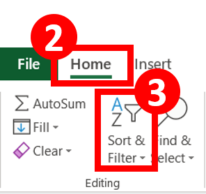
Step 2: In “Home” tab, select “Sort & Filter”
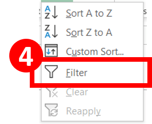
Step 4: Select “Filter“
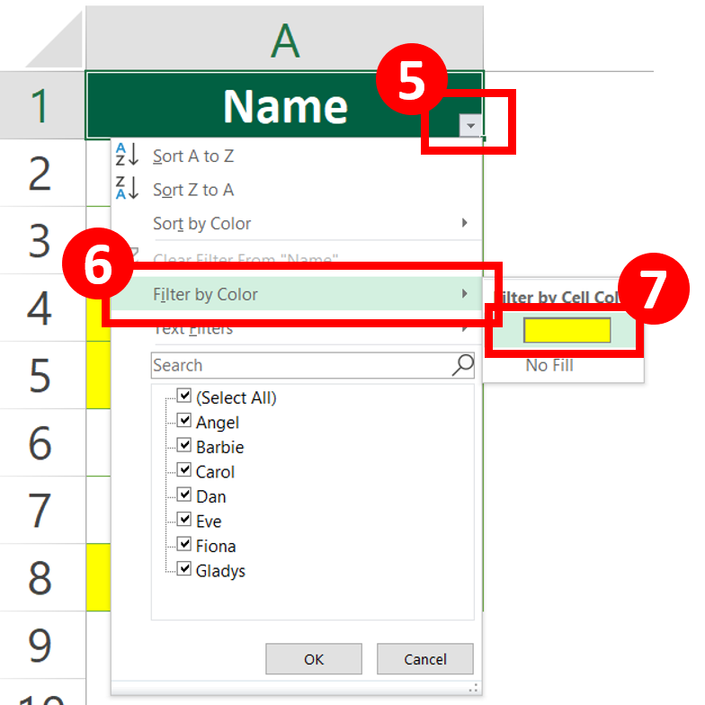
Step 5-7: Press the small triangle, select Filter by Colour and the colour you have
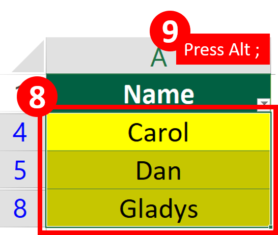
Step 8-9: Select cells with colour and press Alt ;
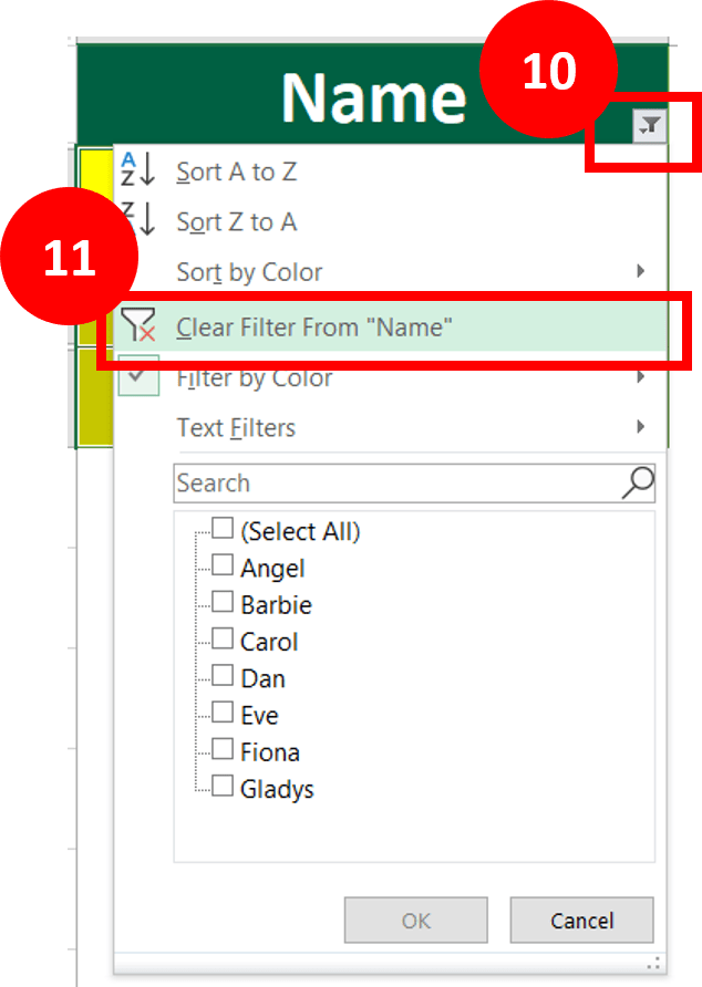
Step 10-11: Press the small triangle, select Clear Filter From “Name”
Step 12: Done

Option 2: Find & Select
Step 1: Press Ctrl + F to open the “Find and Replace” dialog
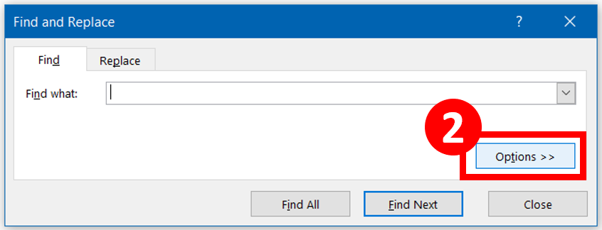
Step 2: Press “Options >>” to enable advanced options
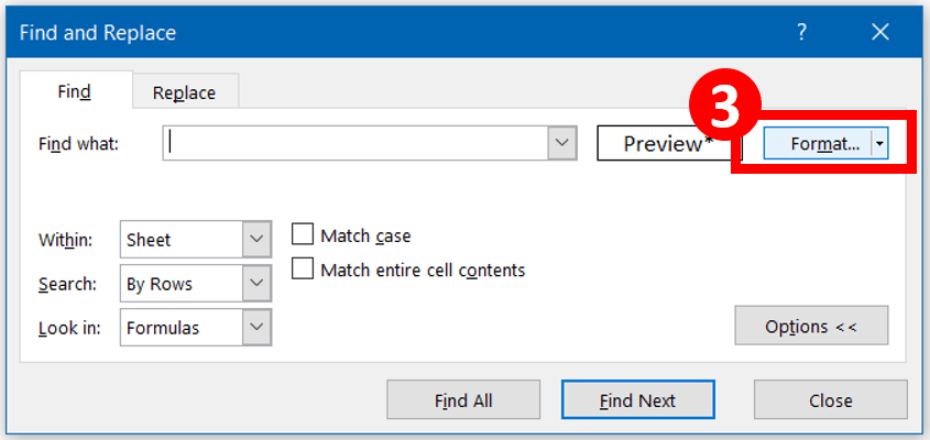
Step 3: Press “Format“
Normal search function only allow you to search by matching text.
Advanced search function allows you to search by matching format.
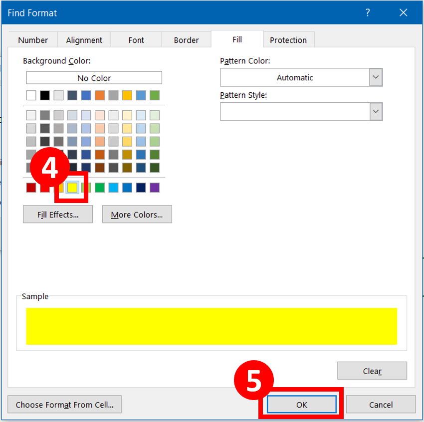
Step 4-5: Select the colour and press “OK”
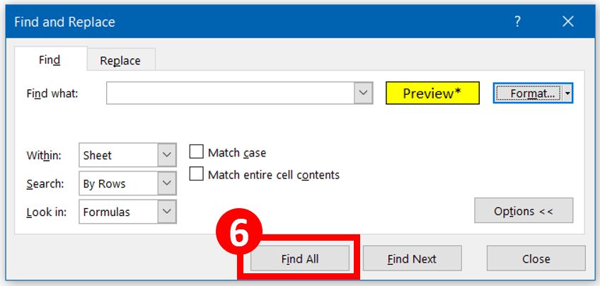
Step 6: Press “Find All“
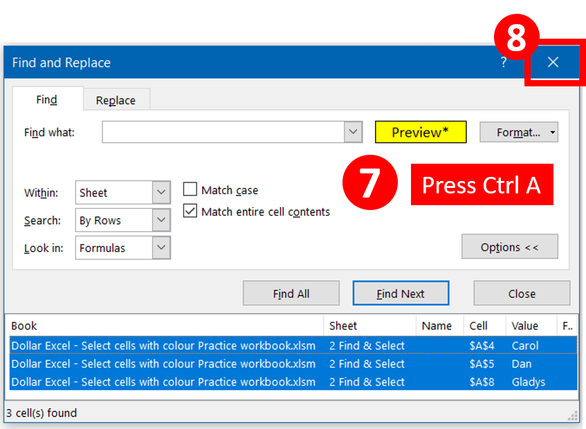
Step 7-8: Press Ctrl A to select all matched results. Close the Find & replace dialog.
Step 9: Done.

Option 3: Sort by Colour
Step 1: Select the column header

Step 2: In “Home” tab, select “Sort & Filter”

Step 4: Select “Filter“

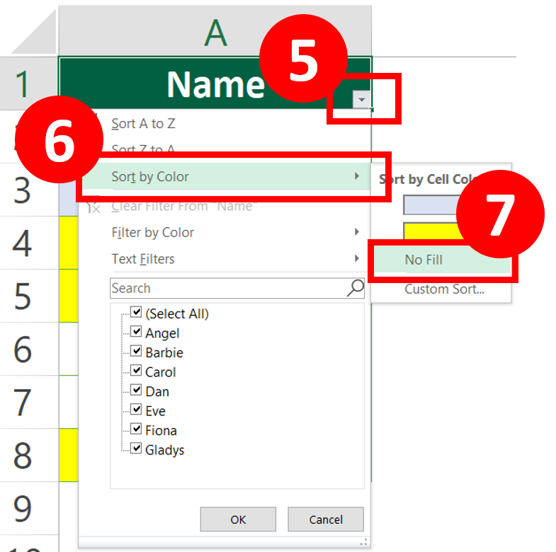
Step 5-7: Press the small triangle, select Sort by Colour and No Fill
This step put all the cells without colour on top.
This step put all the cells without colour on top.
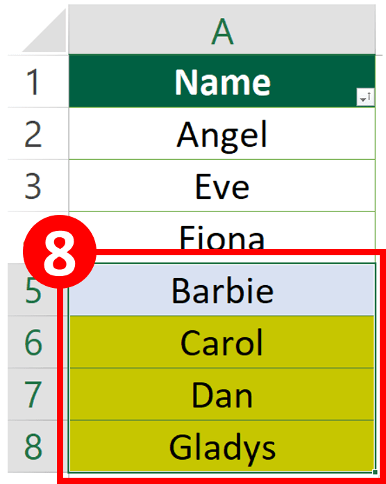
Step 8: Select the cells with colour
Option 4: VBA
Read How to Insert & Run VBA code in Excel – VBA101 if you don’t know how to use the VBA code.
Step 1: Select the cell range
Step 2: Apply this VBA code
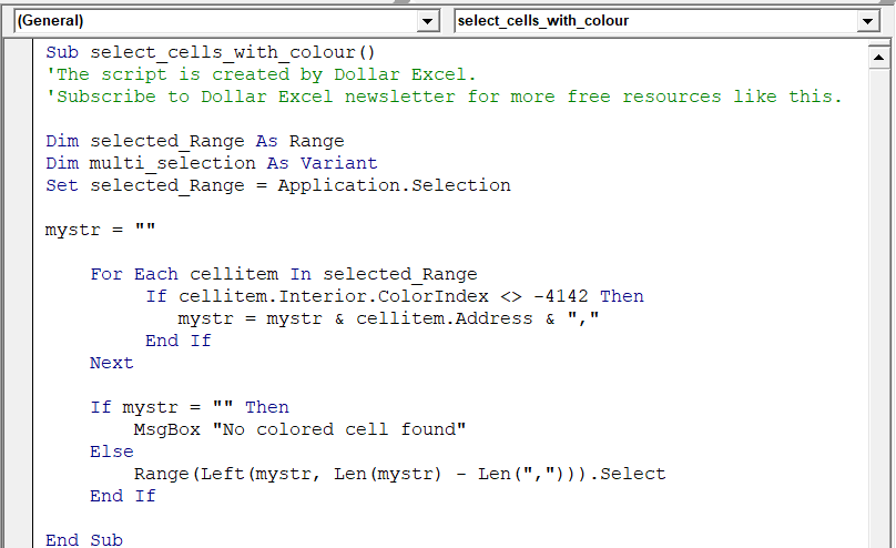
Sub select_cells_with_colour()
'The script is created by Dollar Excel.
'Subscribe to Dollar Excel newsletter for more free resources like this.

Dim selected_Range As Range
Dim multi_selection As Variant
Set selected_Range = Application.Selection

mystr = ""

    For Each cellitem In selected_Range
         If cellitem.Interior.ColorIndex <> -4142 Then
            mystr = mystr & cellitem.Address & ","
         End If
    Next

    If mystr = "" Then
        MsgBox "No colored cell found"
    Else
        Range(Left(mystr, Len(mystr) - Len(","))).Select
    End If

End Sub
What this code will do
- It will select cells with colour
- If none of the selected cells are filled with colour, it will show “No colored cell found”
The logic of the code
- Identify cells with colour
- Assign the cell address of cells with colour to an array
- It will select the cells those cells in array
Customize your VBA code
To select cells with no background colour
If cellitem.Interior.ColorIndex = -4142 ThenDo you find this article helpful? Subscribe to our newsletter to get exclusive Excel tips!


