Sometimes we have to insert bracket in Excel cells.
The easiest way to wrap text in bracket is to manually input it. This process may take an hour if you have thousands of rows. Not only is the manual process time consuming, but also more prone to errors.
Is there any other way to reduce our workload and likelihood to make mistakes?
In this article, I will show you 3 ways to add bracket to Excel cells. They are by formula, number format and VBA respectively.
Each of the method has its advantages and disadvantages. To help you make a better choice, I have made a summary table below. You can take a look at the pros & cons table first to see which method fits you the most.
Pros & cons of each method to insert bracket in Excel
| Method | Advantage | Disadvantage |
|---|---|---|
| Formula | Dynamic | You need another column for operation |
| Number format | You don’t need another column | / |
| VBA | Fastest once script is written | Cannot be undone |
Insert Bracket In Excel Cells Example
In this article, I will show you how to wrap text inside the bracket.
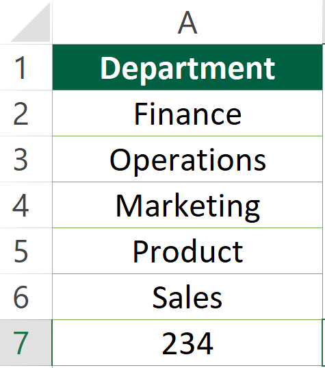
Sample Workbook
Download the workbook to practice it by yourself!

Expected Outcome
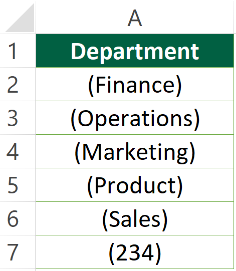
Insert Bracket In Excel Cells By formula
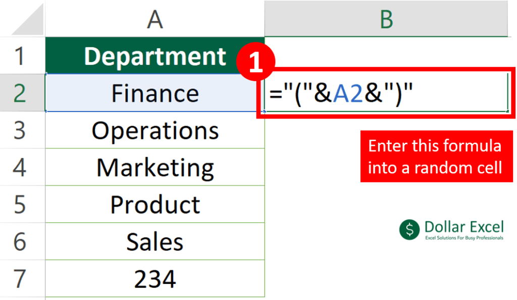
Step 1: Enter this formula into a random cell
Step 2: Drag the formula down
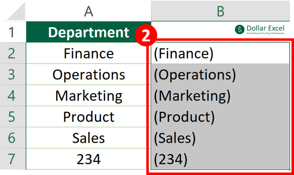
Step 3: Done
Insert Bracket In Excel Cells By number format
Step 1: Select the cell to insert bracket
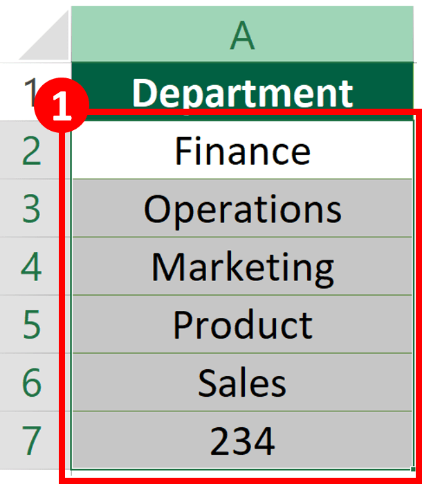
Step 2: Open the “Format Cells” dialog

Step 3: Select “Custom”, type this into format box and press “OK”
"("General")";"("@")"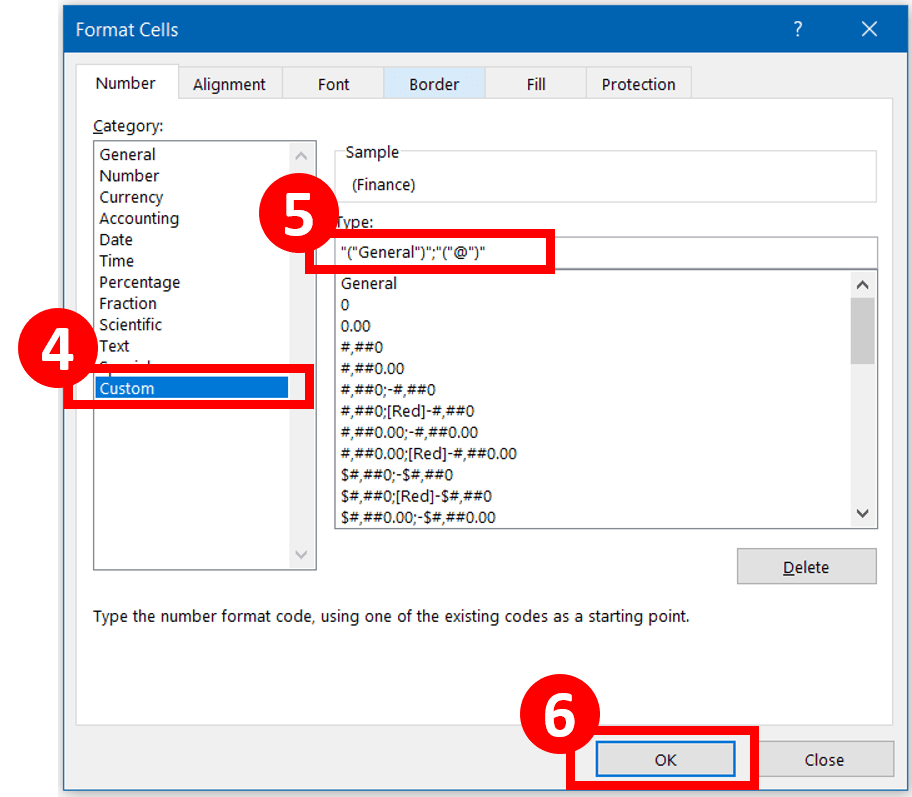
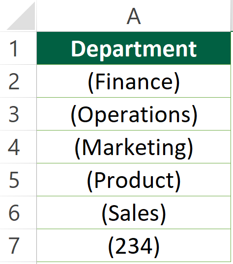
Step 4: Done
Option 3: By VBA
Read How to Insert & Run VBA code in Excel – VBA101 if you don’t know how to use the VBA code.
Step 1: Select the cell to insert bracket

Step 2: Paste the following script
Sub Insert_bracket()
'The script is created by Dollar Excel.
'Subscribe to Dollar Excel newsletter for more free resources like this.

For Each Cell In Selection
Cell.Value = "(" & Cell & ")"
Next

End Sub
Step 3: Run it
Do you find this article helpful? Subscribe to our newsletter to get exclusive Excel tips!


