Background
Excel has over 1 million rows and more than 10000 columns. Sometimes the navigation between different cells can be difficult and quite time-consuming.
Although you might have more than 10000 cells, most of the time there are only a few cells that are important. For example in an income statement, gross income and expenses could be the things you care the most. Rest of the cells may contain some raw data but they are not as important.
What can we do to make our life easier?
If you have the following questions, make sure you keep reading.
- How to quickly jump to a specific cell
- How to create buttons to open/go to certain sheets in Excel
- How to jump to a Specific Cell Using a Hyperlink
In this article, I will show you how to create jump to cells button in Excel. With those button, worksheet navigation becomes a lot easier.
Example
In this article, we will use the Monthly expense table as an example.
As you can see, there are three buttons in the top left corner, namely “Total”, “2019 Jan FB marketing” and “2019 Oct IG marketing”.

Pressing these buttons will bring you to its corresponding cell.
“Total” will bring you to cell H15.
“2019 Jan FB marketing” will bring you to cell E3.
“2019 Oct IG marketing” will bring you to cell F12.
To better demonstrate the usage of the button, the active cell is highlighted in yellow using VBA.
Sample Workbook
Download the workbook to practice it by yourself!

Step-by-step Tutorial
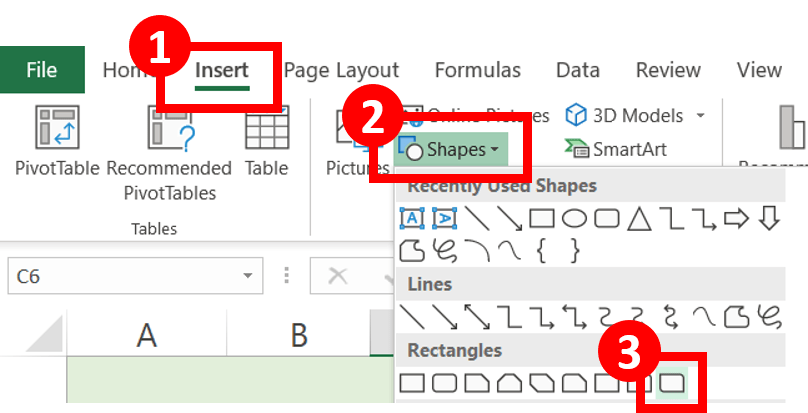
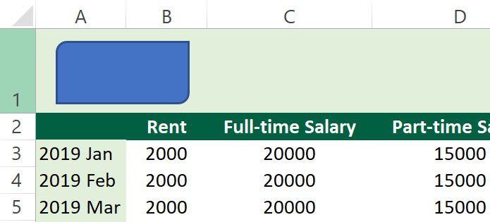
Step 1-3: In Insert tab, select Shapes and choose any shape
You are free to select any shapes. In this example, I will use the corners rounded rectangle. I personally prefer rectangle if I am going to put text inside the button. If you don’t, you can go for circle.
Here is the one I made just now.
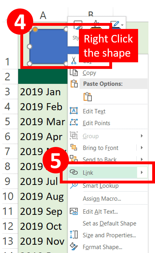
Step 4-5: Right click the shape and press “Link”
This will open the “Insert Hyperlink” dialog.
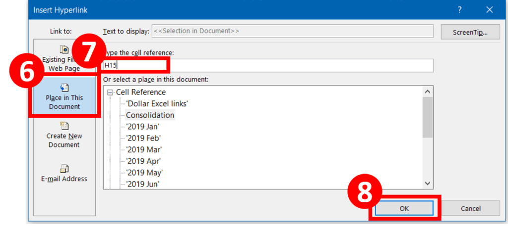
Step 6: Select Place in This Document
As you can see from the left panel, there are a total of 4 options.
- Existing File or Web page
- Place in This Document
- Create New Document
- E-mail Address
In this tutorial, we will be using “Place in This Document”.
As suggested by its name, this option allows you to link to a place in the current workbook.
Step 7: Input cell address in “Type the cell reference: “
In this example, I would to link the button to the Total expense (Cell H15).
Step 8: Press “OK”
Step 9: Format your shape
You can change the background colour, border, height, etc.

Step 10: Input whatever text you want
You can’t just press the button to edit the text.
You have to first right click the button and then double click it.

Step 11: Done
Do you find this article helpful? Subscribe to our newsletter to get exclusive Excel tips!