How To Auto Change Sheet Reference In Copied Formulas?

Background

Are you facing the below situation?

” I would like to copy the formula down and each cell will be referencing different worksheets. For instance, cell B1 will be referencing Sheet A, cell B2 will be referencing Sheet B. I have 200 hundred rows of data. Is manually changing the reference sheet the only way out?”

In this article, I will show you how to reference worksheet dynamically using the INDIRECT function.

Example

Sample Workbook

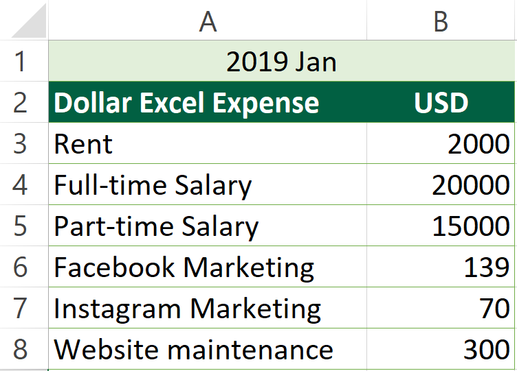
In this article, I will be using Dollar Excel expense table in 2019 as an example. You can download it at the end of this article.

In the example, there are 12 tabs in total. Each tab contains the expense table of Dollar Excel throughout the year 2019. They are all of the same formats.

You can download the workbook to practice it by yourself.

You may also be interested in How to Display the Formula as Text in Excel?

What we want to achieve

I would like to make a new tab called “2019 summary”. This tab will consolidate expense information for the year 2019 and allows me to understand my expense structure at a quick glance.

This screenshot shows the expense table of 2019 January. This serves as an example to understand the format of the table. — Remaining 11 months’ data are also in this format

Each tab contains the expense table of the specified month

Expected Outcome

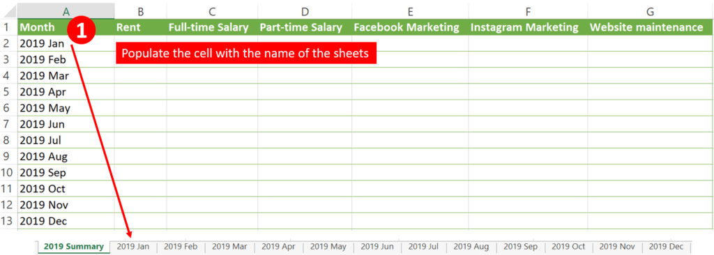
This is how the summary tab looks like.

This one tab consolidated “Rent”, “Full-time Salary”, “Part-time Salary”, “Facebook Marketing”, “Instagram Marketing”, “Website maintenance” for every month in year 2019.

This table is the result we would get following the step I will teach you in this tutorial — The outcome will be like this

You may also be interested in How to Sum Intersections of Multiple Ranges (Excel)

INDIRECT function

The INDIRECT function returns the reference specified by a text string.

In other words, it converts a text string into a valid reference.

Syntax of INDIRECT function

Ref_text is a reference to a cell that contains an A1- or RICI -style reference, a name defined as a reference, or a reference to a cell as a text string.

INDIRECT (ref_text, [a1])

How to use INDIRECT function

Consider which worksheet to reference
Put the name of your worksheet in a cell
Use INDIRECT function to reference the sheet name and the cell

Step-by-step Tutorial

Step 1: Populate Cell A2 to Cell A13 with the name of the worksheets

You may also be interested in Look Up the Last Value in Column/Row in Excel

Step 2: Populate Cell B2 with this formula

=INDIRECT("'"&$A2&"'"&"!"&"B3")

The formula above reduces to

=INDIRECT('2019 Jan'!B3)

The above formula is equivalent to

='2019 Jan'!B3

Step 3: Populate other cells with similar formula

Formula of Cell C2:

=INDIRECT("'"&$A2&"'"&"!"&"B3")

Formula of Cell D2:

=INDIRECT("'"&$A2&"'"&"!"&"B4")

Formula of Cell E2:

=INDIRECT("'"&$A2&"'"&"!"&"B5")

Formula of Cell F2:

=INDIRECT("'"&$A2&"'"&"!"&"B6")

Formula of Cell G2:

=INDIRECT("'"&$A2&"'"&"!"&"B7")

You may also be interested in Look Up the Last Value in Column/Row in Excel

Step 4: Drag the formula down to remaining cells

And we are done!

Hungry for more useful Excel tips like this? Subscribe to our newsletter to make sure you won’t miss out on any of our posts and get exclusive Excel tips!