Applying serial number in a filtered list is a thorny problem. If you hard code the serial number or use the autofill function, the number will be renumbered automatically. In that case, you will have to manually change the number again.
In this article, I will show you two ways to apply serial number after filter. The first way is to add a new column of serial number and the second way is to make the serial number renumber automatically.
Sample
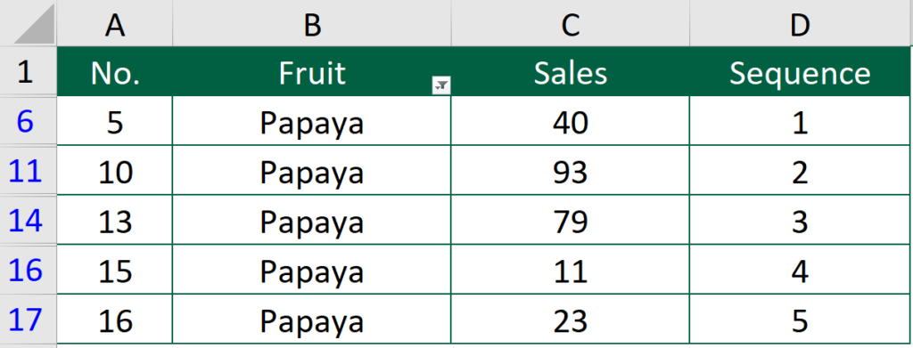
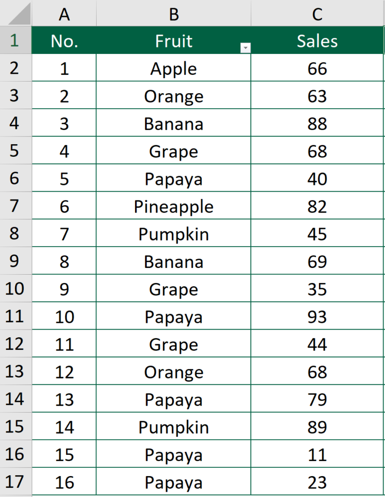
What we would like to do
To have number sequence when the filter is applied
You might also be interested in Edit The Same Cell In Multiple Excel Sheets
Apply serial number after filter in Excel by adding a column
Step 1: Apply the filter as usual
In this case, I only kept the “Papaya” in the column.
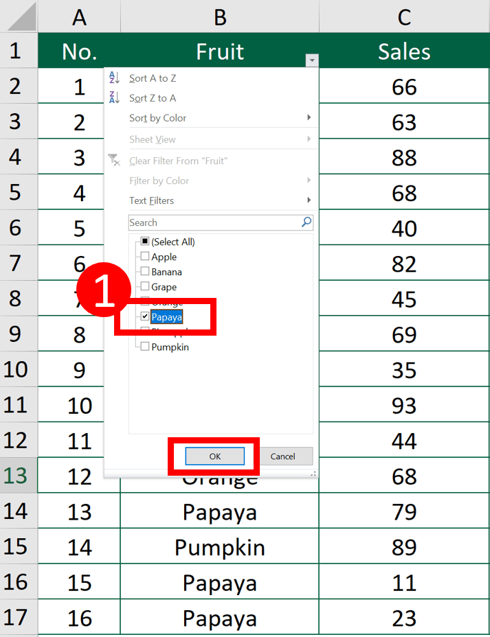
Step 2: Add a new column
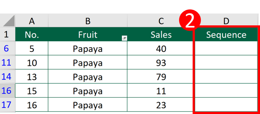
Step 3: Enter this formula in Cell D6
=COUNTA($D$1:D5)
In this example, I will enter the formula in cell D6. You will have to adjust the formula a bit when you use it.
If the condition is like this:
- you are entering the serial number in column B,
- the first cell of the sequence is in row 11,
Then the formula will be like this
=COUNTA($B$1:B10)
Step 4: Copy the formula down
You might also be interested in How to split Excel sheets into separate workbooks
Apply serial number that will renumber automatically
The beauty of this method is that you don’t have to repeat the above process when the filter is changed. After you applied the formula below, the serial number will renumber automatically.
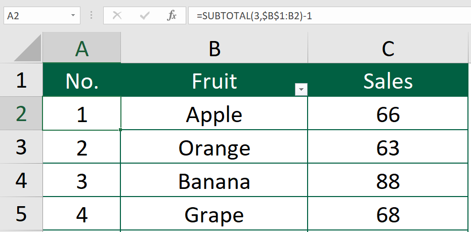
Step 1: Enter this formula in cell A2
=SUBTOTAL(3,$B$1:B2)-1
If the serial number is in column G, then you should change the above formula to =SUBTOTAL(3,$H$1:H2)-1.
Step 2: Copy the formula down
For example, the formula in cell A3 should be =SUBTOTAL(3,$B$1:B3)-1
What will happen when filter is applied
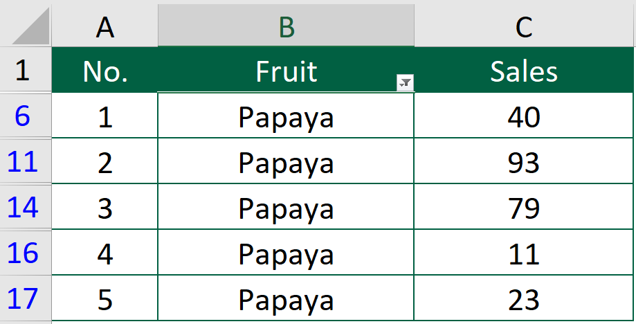
Let’s say I would like to display “Papaya” only.
The number in column A will renumber automatically.
Hungry for more useful Excel tips like this? Subscribe to our newsletter to make sure you won’t miss out on any of our posts and get exclusive Excel tips!


