


This tutorial is part 1 of the Binomial Option Pricing Tutorial Series. For part two, please go to Binomial Option Pricing (Excel VBA).
When it comes to quantitative trading, a great tool to hedge your investment risks is to buy/sell options on the market. For example, if you want protection on your long positions against market downturns, you could buy a put option on the market index. That way, when the market goes south, the value of your put option can compensate for your loss on the long positions.
To price an option contract, we rely on what we called “Financial Models”. A financial model is basically an application to a certain set of assumptions that help us derive general principles in obtaining a fair value of financial instruments. A key assumption underlying option pricing is the principle of no-arbitrage. The no-arbitrage principle dictates that the price of 2 financial instruments with the same payoff should have the same price – this allows us to use what we call a “replicating portfolio” to price the options. We will use this principle extensively through our discussion.
We are going to first explore a more naïve model, the binomial option pricing model.
No arbitrage pricing means that 2 instruments with the same payoff structure should have the same price.
A very rough review of European options
European options give the right to the long side (option-holders) to either buy (call) or sell (put) the stock at a pre-specified price (K) at the end of the option contract. Taking a call option as an example, at maturity, if the price is higher K we’ll exercise the option and buy the now-expensive stock at a cheap price (K); likewise, if the price is lower than K the option is of no value to us. Therefore, the payoff of holding call options is MAX(S – K, 0), meaning that the value of the option contract is S – K (difference of current stock price and the strike price) if S is greater than K, otherwise the value is 0. You can also sell an option, but this time you will have the obligation, not the right to exercise the option. If you short a call option, you’ll need to pay the long-side for S – K if S is greater than K, but you can get away with it and pay nothing if S is less than K at maturity of the contract.
Binomial Option Pricing Model
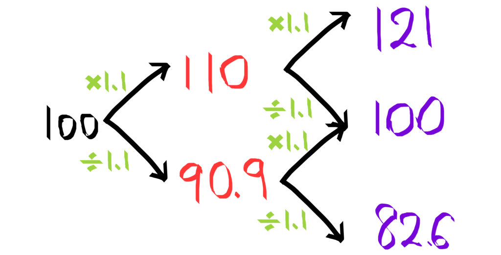
The binomial option pricing is a very simplified model of option pricing where we make a fundamental assumption: in a single period, the stock price will go up or down by a fixed percentage. For example, if our stock is $100 today, it will either go up to $110 tomorrow or $90.9 tomorrow, with no other possibilities. Because we know the call option payoff definitely for both scenarios (e.g. assuming strike price is $100, the payoff is $10 or nothing, respectively), what remains is an appropriate price for the call option today.
To find that, we use a replicating portfolio that has d unit of stocks and short a call option. This replicating portfolio is a hedged portfolio because if the stock price goes up, our gain is limited by shorting the call option (recall that we’ll pay the long-side if S > K). There exist a specific value of d, which we can call d*, such that if you hold d* unit of stock and short a call option, you’ll always get the same payoff regardless of whether the stock actually goes up or down.
The key idea here is that if you get the same payoff regardless of the market, your investment is risk-free you should only be paid the risk-free interest rate, by the principle of no-arbitrage. Therefore, you can come up with a value of your replicating portfolio (d* unit of stock and short a call option) by discounting your risk-free payoff with the risk-free interest rate, and back out the value of the call option!
Find a replicating portfolio that is risk-free.
Sample Workbook
Let’s see this in action in our next section, and feel free to download this workbook to follow through with our examples!
Using Excel formula (2-period)
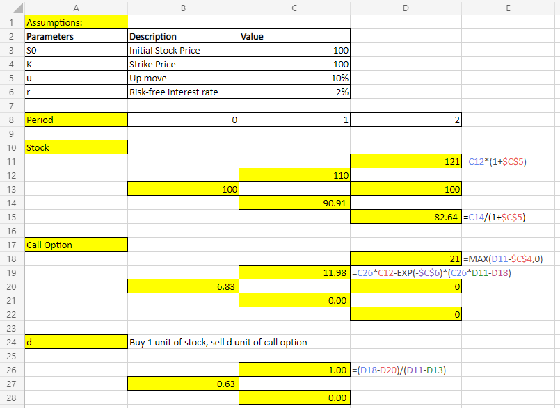
To price a European call option for a 2-period, we use what we call a Backward Analysis, i.e. we first look at what happens at maturity, then work backward to calculate the price of the call option as of today. Using the formula =MAX(S – K,0) in cell D18 to D22, we calculate the option value at maturity should the stock price turns out to be any of these: {121,100,82.6}. Next, we compute d*, the unit of stocks needed such that our replicating portfolio is risk-free in cell C26 to C28. Lastly, using d*, we compute the value of the portfolio at Period=1 by discounting the portfolio value at Period=2 with exp(-r), where r is the risk-free interest rate.
We repeat this analysis for all the nodes and periods involved, which finally yields us $6.83, today’s appropriate option value. Of course, we can extend this to more than 2 periods, but here is where Excel VBA can do the heavy-lifting for us. Read our next article to learn more about option pricing with VBA!
Do you find this article helpful? Subscribe to our newsletter to get regular Excel tips and exclusive free Excel resources.