Very often we need to get distinct or unique value from a column in Excel. In SQL, it is as simple as Select Distinct. However, we don’t have such thing as Select distinct in Excel. What should we do?
No worries at all! There are a couple of ways to get distinct values in Excel.
In this article, I will show you 6 different ways. They are “Remove duplicates”, “Advanced filter”, “Function”, “Formula”, “Pivot table” and “VBA” respectively.
These ways allow you to deal with almost all kinds of situation when it comes to getting unique values in Excel.
You may also be interested in How to Generate Random Dates in Excel
Example
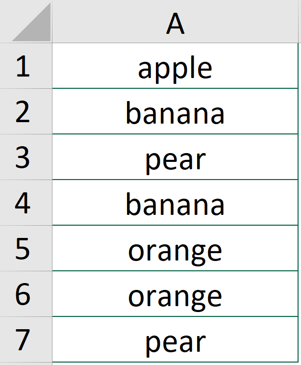
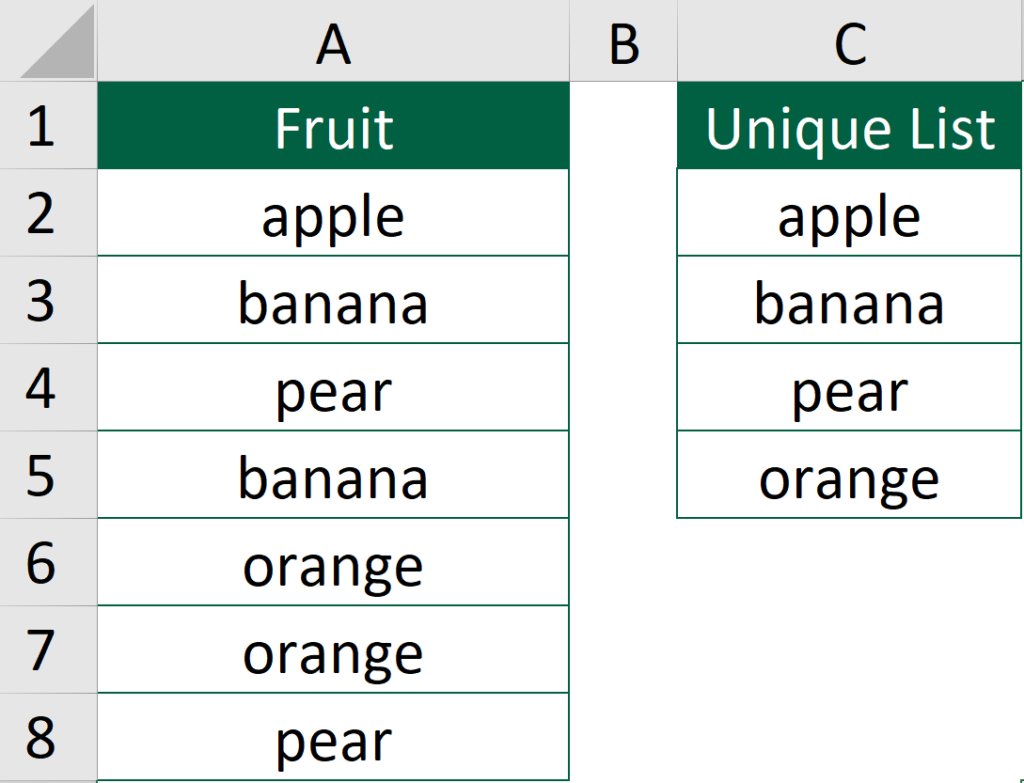
In this article, we will be using the following list as an example.
On the list, there are “apple”, “banana”, “pear”, “banana”, “orange”, “orange” and “pear” respectively.
Among the list of value, there are a few number of duplicates.
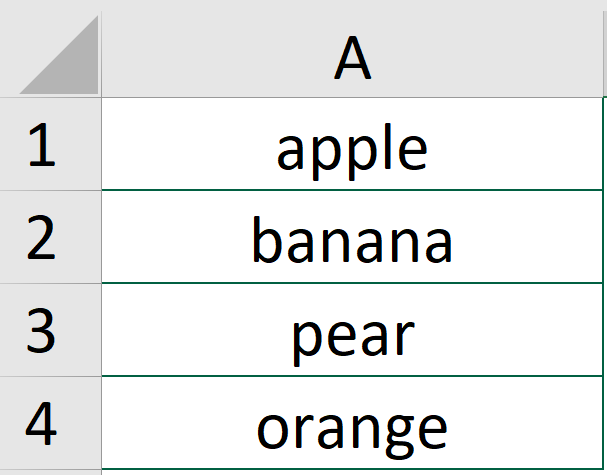
If we are to get the distinct value from the list, they would be “apple”, “banana”, “pear” and “orange”.
It is easy to spot the distinct value if the list is short but that is usually not the case. That is why we will need the following solutions.
Get distinct values in Excel by Remove Duplicates
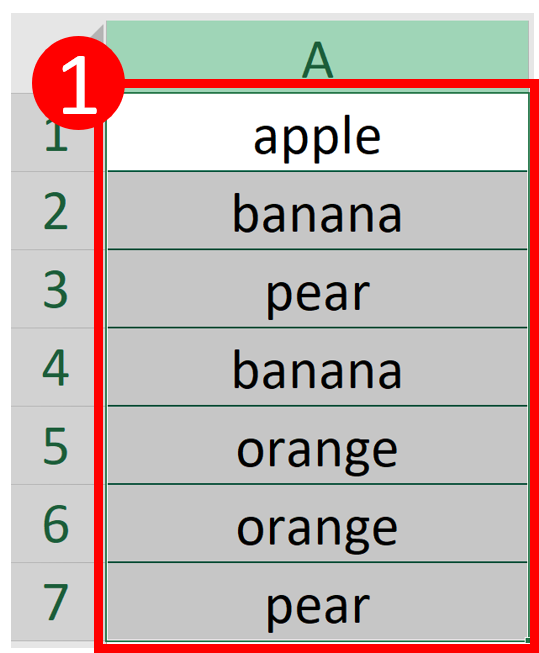
Step 1: Select the data range
Step 2: Select Remove Duplicates

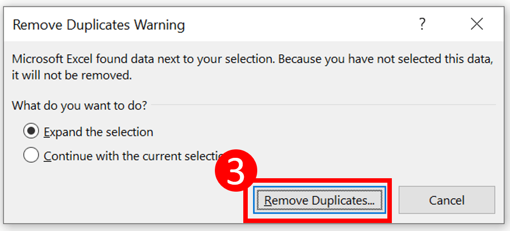
Step 3: Press Remove Duplicates
Result
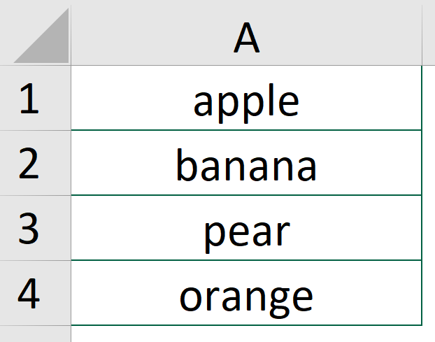
Get distinct values in Excel by Advanced Filter
Step 1: Select the data range

Step 2: Select Advanced

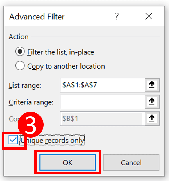
Step 3: Check Unique records only and press OK
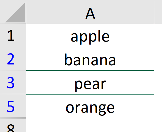
Result
You may be interested in How To Center Cells Across Multiple Columns?
Get distinct values in Excel by Function
UNIQUE function Syntax
UNIQUE(array, [by_col], [occurs_once])
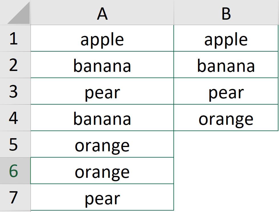
Formula of Cell B1
=UNIQUE(A1:A7)
Result
You may be interested in How To Reverse Concatenate In Excel (3 ways)?
Get distinct values in Excel by By Formula
UNIQUE function is purposefully made to get a distinct list of values. The only downside is that UNIQUE() is currently available in certain version of Excel. Not every Excel users get to use this wonderful function.
Fortunately, we can use a formula to replicate the UNIQUE function. The formula is a bit long yet not as complicated as many people think.
To get a better understanding of this formula, you may want to check out How to Get Unique Values Without Unique function? The article explains the formula in details.
Standard Formula
=IFERROR(INDEX($A$2:$A$9,MATCH(0,INDEX(COUNTIF($C$1:C1,$A$2:$A$9),0,0),0)),"")
Array Formula
=IFERROR(INDEX($A$2:$A$9, MATCH(0, COUNTIF($C$1:C1, $A$2:$A$9), 0)), "")
Result
You may be interested in How to Sum Intersections of Multiple Ranges?
Get distinct values in Excel by By Pivot table
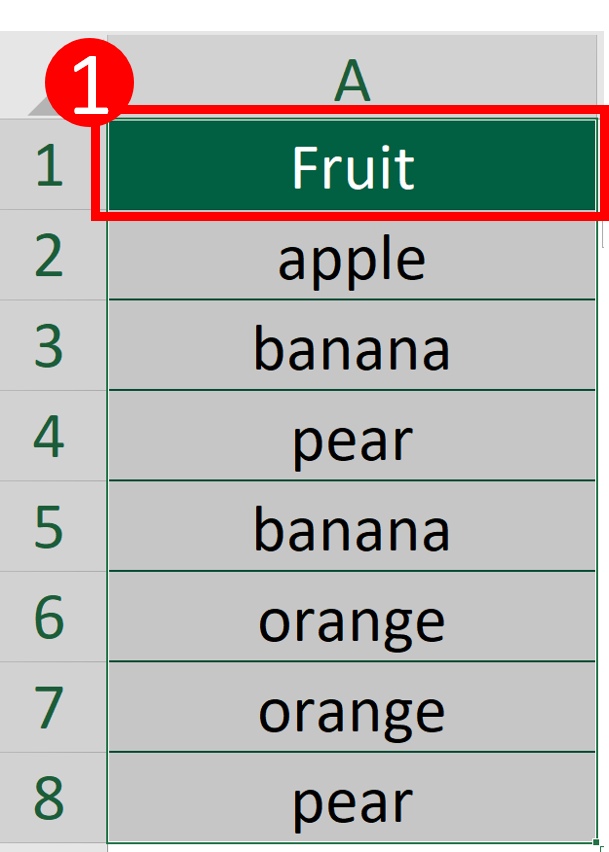
Step 1: Select the data range
Make you give your data range a header or things may go wrong.
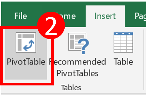
Step 2: Select PivotTable
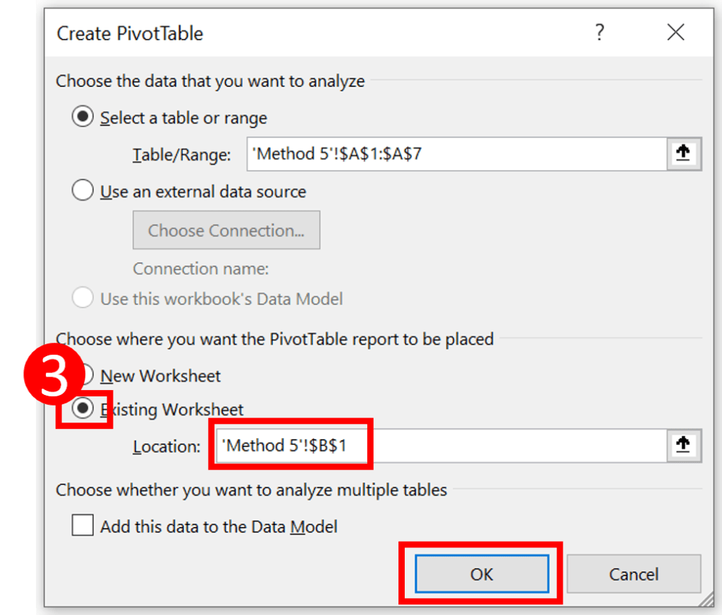
Step 3: Select Existing Worksheet, choose a location and press OK
I selected cell B1 as the location.
Now your Excel should become like this.
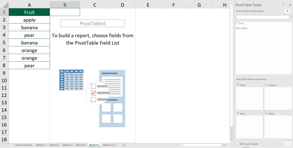
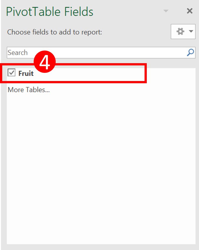
Step 4: Select the field
The top cell in your data range will be perceived by Excel as the name column header.
By selecting “Fruit”, you are basically telling Excel “Please show the column in my PivotTable”.
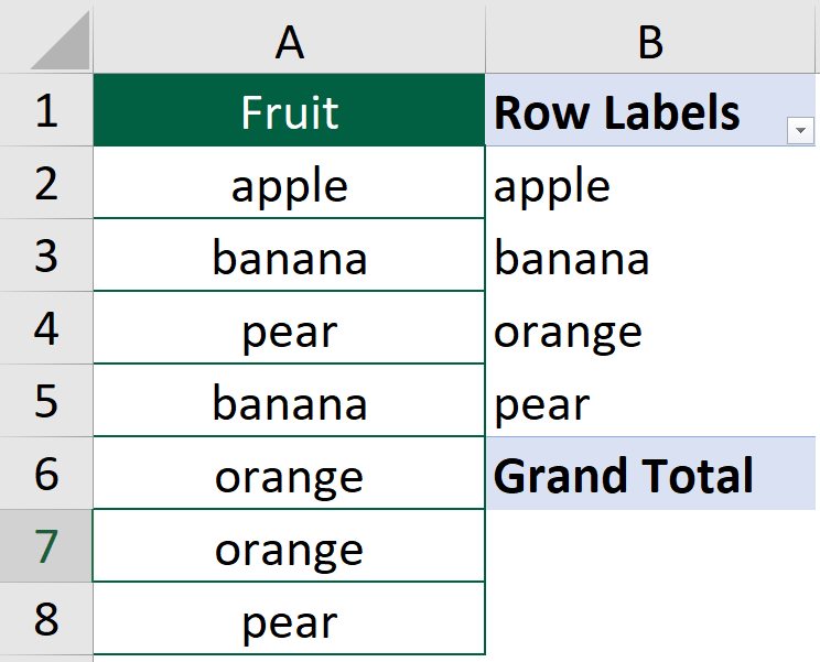
Result
The PivotTable automatically shows distinct values only.
You may be interested in How to use REPT functions to the Most.
Get distinct values in Excel by VBA
Check out How to Insert & Run VBA code in Excel – VBA101 to see why you should learn VBA.
So basically we are trying to do the following things:
- Identify cells that are not unique
- Delete those cells
Below are the code that does the things we suggested above.
How to use the code
Step 1: Select cell ranges
Step 2: Run the code
Sub GetDistinctvalue()
    'perform the code only when the active cell is not equal to zero
    Do While ActiveCell.Value <> ""
        'If the value of the cell in loop is equal to any of the cell selected
        If ActiveCell.Value = ActiveCell.Offset(1, 0).Value Then
            'Select the active cell
            ActiveCell.Select
            'Delete it and move the remaining cells upward so there should be no blank cell
            Selection.Delete Shift:=xlUp
        Else
            'Make the next cell in selection active
            ActiveCell.Offset(1, 0).Activate
        End If
    Loop
End Sub
Result

You may be interested in How to use REPT functions to the Most.
Hungry for more useful Excel tips like this? Subscribe to our newsletter to make sure you won’t miss out on any of our posts and get exclusive Excel tips!


